The Hydrophobic Effect in Protein Folding: From Fundamental Driver to Therapeutic Applications
This article provides a comprehensive exploration of the hydrophobic effect as a central driving force in protein folding, synthesizing foundational principles with current research debates and methodological advances.
The Hydrophobic Effect in Protein Folding: From Fundamental Driver to Therapeutic Applications
Abstract
This article provides a comprehensive exploration of the hydrophobic effect as a central driving force in protein folding, synthesizing foundational principles with current research debates and methodological advances. It examines the historical context and thermodynamic basis of hydrophobicity, critiques the classical 'oil drop' model in light of modern structural data, and discusses the competing roles of backbone solvation and side-chain interactions. The content further details computational methods for predicting hydrophobicity and folding, explores challenges in force field accuracy and sampling, and validates concepts through applications in drug discovery, particularly in targeting protein-protein interactions. Aimed at researchers and drug development professionals, this review connects fundamental biophysical principles to therapeutic design, highlighting future directions for the field.
The Hydrophobic Effect: Unraveling the Fundamental Driver of Protein Folding
The hydrophobic effect is widely recognized as a fundamental driving force in protein folding, molecular recognition, and drug design [1] [2]. This in-depth technical guide traces the historical development of this concept from its initial empirical observations in anesthesia to its formalization as a quantitative principle in biochemistry. The journey begins with the seminal work of Meyer and Overton, who first correlated lipid solubility with biological activity, and culminates with Kauzmann's profound insight into the role of "hydrophobic bonds" in stabilizing protein structures [2] [3]. Understanding this historical progression is essential for researchers and drug development professionals seeking to comprehend the physical forces that govern biomolecular interactions and stability. This document frames these developments within the broader context of protein folding research, examining both the classical theories and emerging challenges to established paradigms.
The Meyer-Overton Era: Foundations in Anesthesia Research
Empirical Beginnings and Historical Context
At the turn of the 20th century, Hans Meyer and Charles Overton independently made a crucial discovery that would lay the groundwork for understanding hydrophobic interactions in biological systems. Their research, conducted between 1899 and 1901, demonstrated a striking correlation between the lipophilicity of chemical compounds and their anesthetic potency [2] [4]. This Meyer-Overton rule proposed that the effectiveness of an anesthetic agent was directly proportional to its lipid solubility, suggesting that these substances exerted their effects by interacting with lipid components of biological systems [4]. This represented one of the first quantitative relationships established between a compound's physicochemical properties and its biological activity.
Experimental Basis and Methodological Approaches
The experimental foundation of the Meyer-Overton rule was based on partition coefficient measurements, which quantified how a compound distributes itself between oil and water phases [2]. Although the exact methodologies employed by Meyer and Overton were not explicitly detailed in the search results, their work established the fundamental principle that biological activity could be predicted by a simple physicochemical parameter - the preference of a compound for a nonpolar environment over an aqueous one. This observation was particularly remarkable given that the molecular structures of neuronal membranes and proteins were unknown at the time. Their findings suggested that anesthetic potency was primarily determined by a compound's ability to dissolve in hydrophobic environments, implicitly highlighting the importance of water exclusion in biological interactions.
Table 1: Key Historical Experiments on Hydrophobic Interactions
| Investigator(s) | Time Period | Key Finding | Experimental System |
|---|---|---|---|
| Meyer and Overton | 1899-1901 | Correlation between lipid solubility and anesthetic potency | Oil-water partitioning |
| Frank and Evans | 1945 | "Iceberg" model of water structure around nonpolar solutes | Thermodynamic measurements |
| Kauzmann | 1959 | Concept of "hydrophobic bond" in protein stability | Protein denaturation studies |
| Némethy, Scheraga, and Steinberg | 1960s | Temperature dependence of hydrophobic interactions | Theoretical modeling |
The Iceberg Model and Early Theoretical Frameworks
Following the observations of Meyer and Overton, the mid-20th century saw significant advances in understanding the molecular basis of hydrophobic phenomena. In 1945, Frank and Evans proposed the "iceberg" model to explain the behavior of water in the presence of nonpolar solutes [1] [2]. According to this model, water molecules form structured "cage-like" arrangements around hydrophobic solutes, resembling the clathrate structures found in gas hydrates [1]. This concept provided a physical explanation for the large negative entropy change observed when nonpolar compounds were dissolved in water.
The iceberg model was subsequently extended to proteins by Klotz, who invoked this concept to explain various biochemical phenomena including pKa shifts, molecular volume changes, denaturation processes, and the altered behavior of protein functional groups in aqueous environments [2]. The key thermodynamic implication was that when hydrophobic molecules associate, some of these structured water molecules are released into the bulk solvent, resulting in an entropy increase that drives the association process [2] [5]. This release of constrained water molecules from the solute-solvent interface to the bulk aqueous phase represented an entropically favorable process that could explain the driving force for hydrophobic associations.
Diagram 1: Frank and Evans' "Iceberg" Model of Hydrophobic Hydration. The association of nonpolar solutes reduces the total structured water shell, releasing water molecules to the bulk and increasing entropy.
Kauzmann's Hydrophobic 'Bond': A Paradigm for Protein Folding
Conceptual Foundation and Terminology
In 1959, Walter Kauzmann published his seminal review article that would fundamentally shape the understanding of protein stability for decades to come [2] [3]. Drawing upon the earlier concepts of Frank and Evans, Kauzmann introduced the term "hydrophobic bond" to describe the attractive interactions between nonpolar groups in aqueous solutions [2]. Kauzmann's profound insight was recognizing that the same principles governing the association of simple nonpolar molecules in water could explain the folding and stability of complex protein structures. His hypothesis proposed that dehydration of nonpolar amino acid side chains, followed by their association in the protein interior, was energetically favorable and represented a dominant factor in thermodynamic protein stability [3].
Thermodynamic Basis and Experimental Evidence
Kauzmann's hypothesis was primarily based on free energy transfer measurements of nonpolar hydrocarbons from water into organic solvents [3]. The negative free energy values observed in these transfer experiments were interpreted as mimicking the energetic changes occurring when nonpolar groups buried in the protein interior during folding. Kauzmann emphasized the entropic contribution to this process, relating it to the structural changes in water molecules surrounding nonpolar surfaces [3]. This "classical" view of hydrophobic interactions as entropy-driven became widely accepted and was incorporated into biochemistry textbooks for decades.
The work of Némethy, Scheraga, and Steinberg further supported and refined Kauzmann's concepts by investigating the temperature dependence of hydrophobic interactions [2]. Their research demonstrated that hydrophobic "bonds" were endothermic - strengthening with increasing temperature up to approximately 60°C - in contrast to hydrogen bonds which weaken with rising temperature [2]. This differential temperature dependence suggested a delicate balance of forces in protein stability, with hydrophobic interactions dominating at higher temperatures while hydrogen bonds maintain structure at lower temperatures.
Table 2: Thermodynamic Characterization of Hydrophobic Interactions
| Property | Characteristic | Molecular Interpretation |
|---|---|---|
| Driving Force | Primarily entropic at room temperature | Release of structured water molecules into bulk |
| Temperature Dependence | Strength increases to ~60°C | Enhanced breakdown of water structure |
| Entropy Change | Positive (ΔS > 0) upon association | Increased freedom of released water molecules |
| Enthalpy Change | Variable, can be positive or negative | Balance between broken and formed water H-bonds |
Critical Experimental Protocols and Methodologies
The experimental foundation supporting Kauzmann's hydrophobic bond concept relied on several key methodological approaches:
Transfer Free Energy Measurements: This involved determining the free energy change for transferring hydrophobic solutes (such as methane or ethane) from water to a nonpolar solvent or to the pure liquid state. The measured values typically ranged between -8 and -12 kJ mol⁻¹ for hydrocarbons like cyclohexane, providing quantitative estimates of the hydrophobic effect [6] [3].
Protein Denaturation Studies: Researchers employed chemical denaturants (urea, guanidinium chloride) or temperature changes to unfold proteins while monitoring structural changes using techniques like circular dichroism, UV spectroscopy, or calorimetry. These studies revealed correlations between nonpolar surface area exposure and denaturation energetics.
Model Compound Studies: Investigations using small peptides or hydrophobic molecules like benzene derivatives measured association constants in aqueous solutions, demonstrating the tendency of nonpolar groups to cluster in water [6].
Evolution from 'Bond' to 'Effect': Semantic and Conceptual Refinement
Terminology Debate and Evolving Understanding
The term "hydrophobic bond" introduced by Kauzmann initially gained traction in the scientific literature, but eventually faced scrutiny as researchers recognized that the phenomenon differed fundamentally from covalent or ionic bonds [2]. The semantic debate centered on whether the association of nonpolar molecules in water resulted from direct attractive forces between the molecules or was instead an indirect effect driven by water reorganization. Throughout the 1960s and 1970s, the term gradually shifted to "hydrophobic interaction" or "hydrophobic effect" to better reflect the underlying physical chemistry [2].
This conceptual evolution was significantly advanced by Robert Hermann's theoretical work in the 1970s, which provided a mathematical framework for understanding hydrophobic phenomena based on surface area and solubility relationships [2]. Hermann proposed that the free energy for hydration of a hydrophobic molecule was linearly related to the number of water molecules that could pack around it, establishing quantitative relationships between hydrophobic surface area and aqueous solubility [2].
Quantitative Frameworks and Hydrophobicity Scales
The development of quantitative hydrophobicity scales represented a critical advancement in applying hydrophobic effect principles to protein research. The introduction of the 1-octanol/water partition coefficient (LogP) as a standardized measure of hydrophobicity by Hansch and colleagues provided a universal parameter for predicting molecular behavior in biological systems [2]. This led to the creation of computational methods for estimating LogP values, including:
- Fragment-based methods (e.g., Rekker's method, C-LOGP)
- Atom-based methods (e.g., Ghose-Crippen method)
- Whole molecule approaches (e.g., Molecular Lipophilicity Potential)
These quantitative approaches enabled researchers to predict the hydrophobic character of amino acid side chains and their contribution to protein stability, folding, and molecular recognition events [7] [2].
Modern Computational and Theoretical Approaches
Contemporary Hydrophobicity Scales and Protein Structure Prediction
Modern research has refined our understanding of how hydrophobicity patterns in protein sequences influence tertiary structure. The burial mode model represents a recent phenomenological approach that predicts burial traces in protein domains based on sequence hydrophobicity [7]. This computationally efficient model (requiring less than one second for a 100-300 residue protein on a single CPU) incorporates hydrophobic effect, steric repulsion, and polymeric constraints as key folding drivers [7]. Parameter optimization studies have demonstrated that classic hydrophobicity scales like Kyte-Doolittle are nearly optimal for predicting residue burial using this model [7].
Challenging Classical Views: Emerging Perspectives
Recent research has begun to challenge Kauzmann's classical hydrophobic interaction hypothesis. A 2021 study by Yoshida and colleagues employed liquid-state density functional theory to calculate solvation free energies in protein folding thermodynamics [3]. Their analysis of the GCN4-p1 leucine zipper formation demonstrated that water-mediated interactions were actually unfavorable for the association of nonpolar groups in the native state, while dispersion forces between nonpolar groups were responsible for their association [3].
This direct interaction mechanism contradicts the long-standing view that avoiding exposure of nonpolar groups to water is the primary stabilizing factor in protein folding. Instead, it suggests that intramolecular direct interactions (van der Waals forces and hydrogen bonds) predominantly stabilize folded proteins, with water-mediated interactions often acting destabilizing [3]. This represents a potential paradigm shift in understanding protein folding energetics.
Diagram 2: Paradigm Shift in Understanding Protein Folding Drivers. The classical view emphasizes favorable water-mediated interactions, while emerging evidence points to direct dispersion forces as key stabilizers, with water-mediated interactions often being unfavorable.
The Scientist's Toolkit: Essential Research Reagents and Methods
Table 3: Key Research Reagents and Methods for Studying Hydrophobic Interactions
| Reagent/Method | Function/Application | Technical Notes |
|---|---|---|
| 1-Octanol/Water System | Standardized system for measuring partition coefficients (LogP) | Universal reference for hydrophobicity quantification |
| Kyte-Doolittle Scale | Hydrophobicity scale for predicting residue burial in proteins | Nearly optimal for burial prediction in phenomenological models |
| Molecular Dynamics Simulations | Atomistic modeling of water behavior near hydrophobic surfaces | Reveals details of water structure and dynamics |
| Liquid-State Density Functional Theory | Ab initio calculation of solvation free energies | Challenges classical views on water-mediated interactions |
| Neutron Scattering | Experimental probe of water structure around solutes | Tests "iceberg" model predictions |
| Bulk Alkanes (methane, cyclohexane) | Model compounds for transfer free energy studies | Provide baseline hydrophobicity measurements |
The historical journey from Meyer and Overton's empirical observations to Kauzmann's conceptualization of the hydrophobic bond represents a foundational narrative in structural biology. This progression demonstrates how simple correlations between lipid solubility and biological activity evolved into a sophisticated understanding of the physical forces governing protein folding and stability. While Kauzmann's hydrophobic bond hypothesis dominated biochemical thinking for decades, recent computational and theoretical advances are challenging this classical view, suggesting a more complex interplay of direct intermolecular forces and water-mediated effects.
For contemporary researchers and drug development professionals, understanding this historical foundation and its ongoing evolution is crucial for interpreting protein behavior and designing molecular interventions. The hydrophobic effect remains a vital concept, but its precise role in protein folding continues to be refined through advanced computational methods and experimental techniques. As research progresses, the integration of these historical insights with emerging paradigms will undoubtedly lead to more accurate models of biomolecular structure and function.
The hydrophobic effect, a fundamental force in aqueous solutions, is primarily an entropic phenomenon driven by the unique properties of water. It describes the tendency of nonpolar substances to aggregate and minimize their contact with water, thereby maximizing the entropy of the surrounding water molecules. This effect is not merely a passive exclusion but an active process governed by the hydrogen-bonding network of water. Within the context of protein folding and biomolecular stability, the hydrophobic effect provides a major thermodynamic driving force for the burial of nonpolar residues, the formation of molten globule states, and the establishment of functional native structures. This whitepaper elucidates the physical chemistry of hydrophobicity, detailing its entropic origin, its dependence on solute size and temperature, and the experimental and computational methodologies employed to quantify its role in directing the folding and function of biological macromolecules.
Hydrophobic interactions are involved in and are believed to be the fundamental driving force of many chemical and biological phenomena in aqueous environments, including molecular recognition, protein folding, and the formation and stability of micelles and biological membranes [1]. The word "hydrophobic" literally means "water-fearing," and the effect describes the segregation of water and nonpolar substances, which maximizes the entropy of water and minimizes the area of contact between water and nonpolar molecules [8]. From a thermodynamic perspective, the hydrophobic effect is defined as the free energy change of water surrounding a solute. A positive free energy change indicates hydrophobicity, whereas a negative free energy change implies hydrophilicity [8].
In biochemistry, the hydrophobic effect is essential to life. It is responsible for the formation of cell membranes and vesicles, the folding of proteins into their native functional three-dimensional structures, the insertion of membrane proteins into lipid bilayers, and the associations between proteins and small molecules [8] [9]. A complete understanding of this effect requires a description of the conformational states of both water and solute molecules across different temperatures, revealing the delicate balance between enthalpy and entropy that dictates solvation behavior [9].
Theoretical Framework: Thermodynamics and Solvation
The Entropic Origin
The classical understanding of the hydrophobic effect is that it is entropy-driven at room temperature. When a nonpolar solute is introduced into water, the water molecules in its immediate vicinity form a structured "cage" or clathrate. The formation of this cage results in a significant loss of translational and rotational entropy for the involved water molecules [8]. The hydrogen bonds between water molecules are reoriented tangentially to the nonpolar surface to minimize the disruption of the bulk hydrogen-bonded network. This structuring leads to a more ordered system and a corresponding decrease in entropy [8] [1].
The aggregation of nonpolar molecules reduces the total surface area exposed to water. This process releases the structured water molecules from the cages back into the bulk solvent, where they experience greater rotational and translational freedom. This release results in a large, favorable increase in the entropy of the system, which is the primary driving force for the hydrophobic effect under standard conditions [8] [1]. The process can be summarized by the fundamental equation of thermodynamics:
ΔG = ΔH - TΔS
Where a positive ΔG indicates hydrophobicity. For the hydrophobic effect, the entropic term (-TΔS) is dominant and favorable for aggregation at room temperature [8] [1].
The Role of Enthalpy and Temperature Dependence
While entropy is the dominant driver at room temperature, the enthalpic component (ΔH) of the hydrophobic effect is also significant and can become dominant under certain conditions. Experimental studies have found that the enthalpic component of transfer energy is favorable, meaning it strengthens water-water hydrogen bonds in the solvation shell [8]. This finding appears counterintuitive but aligns with the observation that hydrophobic interactions can be enthalpy-driven in some binding systems [1] [8].
The hydrophobic effect exhibits a strong temperature dependence. At higher temperatures, when water molecules become more mobile, the energy gain from strengthened hydrogen bonds in the solvation shell decreases along with the entropic component [8]. This temperature dependence is directly responsible for the phenomenon of "cold denaturation" of proteins, where proteins unfold at low temperatures [8] [9]. At lower temperatures, the enthalpic contribution becomes more favorable, stabilizing the unfolded state where more water molecules can interact with the protein backbone and side chains.
The Size Crossover: Small vs. Large Solutes
A critical concept in hydrophobicity is the dependence on solute size. Theoretical and experimental work has revealed a crossover around the 1 nm length scale [1] [9].
- Small Solutes (< 1 nm): For small nonpolar solutes, water molecules can rearrange around the solute without a significant net loss of hydrogen bonds. The hydration free energy scales linearly with the volume of the solute. The water network remains largely intact, forming "iceberg"-like structures around the solute [1].
- Large Solutes (> 1 nm): For large hydrophobic surfaces, water cannot maintain its hydrogen-bonding network at the interface. Hydrogen bonds are broken, resulting in an enthalpic penalty. In this regime, the hydration free energy scales linearly with the surface area of the solute [1] [9].
Proteins present a complex case because their surfaces are mosaics of polar and non-polar residues. Even though proteins are larger than 1 nm, the presence of polar groups allows water at the protein interface to, on average, form the same total number of hydrogen bonds (protein-water + water-water) as bulk water, causing them to effectively behave like small solutes in this respect [9].
Table 1: Thermodynamic Characteristics of Hydrophobic Hydration
| Feature | Small Solutes (<1 nm) | Large Solutes (>1 nm) |
|---|---|---|
| Scaling of Hydration Free Energy | Linear with solute volume | Linear with solute surface area |
| Hydrogen Bonding at Interface | Largely maintained; water can rearrange without breaking H-bonds | Disrupted; H-bonds are broken, leading to an enthalpic penalty |
| Water Ordering | Increased order ("iceberg" model) | Depends on surface chemistry; can be less ordered |
| Dominant Thermodynamic Driver | Entropy (TΔS) | Enthalpy (ΔH) can become significant |
Hydrophobicity in Protein Folding and Stability
A Major Driving Force for Folding
The hydrophobic effect is the principal driving force behind the folding of globular proteins. The process of folding minimizes the number of hydrophobic side chains exposed to water, which stabilizes the folded state [8]. In the native state, proteins typically possess a hydrophobic core in which nonpolar side chains (e.g., valine, leucine, isoleucine, phenylalanine, tryptophan, and methionine) are buried, shielded from the aqueous solvent. Charged and polar side chains are predominantly situated on the solvent-exposed surface, where they can interact with surrounding water molecules [8].
The drive to sequester hydrophobic residues away from water creates a compact, molten globule-like state early in the folding pathway. Subsequent fine-tuning of the structure, including the formation of specific hydrogen bonds and van der Waals contacts within the core, then optimizes the stability of the native fold [8] [8]. While hydrogen bonds within the protein are crucial for stability and specificity, the initial collapse is governed by the hydrophobic effect [8].
Structural Biology: Hot vs. Cold Denaturation
The temperature dependence of the hydrophobic effect provides a unique window into its mechanism, exemplified by the study of hot and cold denatured states. Research on yeast frataxin, a protein for which both states have been characterized, reveals structural differences that underscore the role of water [9].
- Hot Denatured State (HDS): At high temperatures, the denatured state is more compact and richer in secondary structure (e.g., α-helix content of 10%) than the cold denatured state. The radius of gyration (Rg) is smaller.
- Cold Denatured State (CDS): At low temperatures, the denatured state is more expanded, has less secondary structure (α-helix content of 6%), and has a higher polyproline II content. Its radius of gyration is larger [9].
These differences are linked to the behavior of water. The number of hydrogen bonds per water molecule in the bulk decreases with increasing temperature. Remarkably, the total number of hydrogen bonds per water molecule (water-water + protein-water) is nearly identical for bulk water and water at the protein interface across temperatures. In the cold denatured state, the protein expands to allow water to form more hydrogen bonds with it, stabilizing the expanded state through enthalpic gains. This finding indicates that proteins, due to their heterogeneous surface, can behave like "small" solutes, with water maintaining its hydrogen-bonding capacity at the interface [9].
The following diagram illustrates the logical relationships and experimental observations that link the hydrophobic effect to protein denaturation states.
Beyond Thermodynamic Stability: Mechanical Stability
While the hydrophobic effect is a major contributor to the thermodynamic stability of the folded state, its role in mechanical stability—a protein's resistance to being unfolded by force—is different. Steered molecular dynamics simulations have shown that the contribution of hydrophobic interactions to the total resistive force during mechanical unfolding varies between one-fifth and one-third. The rest of the force is attributed primarily to hydrogen bonds [10]. This contrasts with their dominant role in thermodynamic stability and is explained by the steeper free energy dependence of hydrogen bonds on the relative positions of interacting atoms compared to the shallower dependence of hydrophobic interactions [10].
Quantitative Measurement and Prediction
Experimental Methodologies
A range of experimental techniques is used to quantify hydrophobicity and its effects on proteins and other molecules.
- Hydrophobic Interaction Chromatography (HIC): This is a standard method for separating proteins based on hydrophobicity. Proteins with higher surface hydrophobicity interact more strongly with the hydrophobic stationary phase and have longer retention times. HIC is widely used to assess the hydrophobicity of therapeutic antibodies [11].
- Partition Coefficients (log P): The logarithm of the partition coefficient of a solute between a nonpolar solvent (like n-octanol) and water is a fundamental measure of hydrophobicity. It is empirically calculated and widely used in drug design and medicinal chemistry [1] [12].
- Nile Red Staining: This fluorescence-based assay is used to quantify the hydrophobicity of materials, including polymers. The dye's emission spectrum shifts based on the hydrophobicity of its local environment [12].
- Calorimetry: Isothermal Titration Calorimetry (ITC) and Differential Scanning Calorimetry (DSC) are used to directly measure the enthalpic (ΔH) and entropic (TΔS) components of hydrophobic interactions and protein stability [8].
- Spectroscopic Techniques: NMR and vibrational spectroscopy (e.g., Raman, IR) are used to probe the structure and dynamics of water molecules at the interfaces of solutes and proteins [1] [9].
Table 2: Key Experimental Protocols for Assessing Hydrophobicity
| Method | Key Measurement | Application in Research | Technical Considerations |
|---|---|---|---|
| Hydrophobic Interaction Chromatography (HIC) | Protein retention time on a hydrophobic column. | Ranking hydrophobicity of protein mutants (e.g., therapeutic antibodies); protein purification [11]. | Salt concentration modulates effect; requires protein in solution. |
| Partition Coefficient (log P) | Equilibrium concentration ratio in octanol/water. | Quantifying hydrophobicity of small molecules and drug candidates; QSAR modeling [1] [12]. | Gold standard for small molecules; less applicable to large polymers/proteins. |
| Nile Red Staining | Shift in fluorescence emission maximum. | High-throughput screening of polymer hydrophobicity; material science [12]. | Semi-quantitative; requires a calibration curve for different material classes. |
| Calorimetry (ITC/DSC) | Direct measurement of heat change (ΔH). | Decomposing free energy into enthalpic and entropic components of binding or unfolding [8]. | Requires significant sample amounts; instrument sensitivity is critical. |
| Spectroscopy (NMR) | Chemical shifts and relaxation rates of water/protons. | Probing water structure and dynamics at protein interfaces; characterizing denatured states [9]. | Can be technically challenging; provides atomic-level detail. |
Computational and In-Silico Approaches
Computational methods are indispensable for predicting hydrophobicity and understanding its molecular origins.
- Hydrophobicity Scales: These are tables that assign a numerical hydrophobicity value to each amino acid based on experimental data or theoretical calculations. Examples include the Kyte-Doolittle scale, which colors residues from hydrophobic (red, e.g., I, V, L, F) to hydrophilic (blue, e.g., R, K, N) [13]. The performance of these scales in predicting experimental results like HIC retention times varies significantly [11].
- Structure-Based Methods: These methods use the three-dimensional structure of a protein to compute hydrophobicity, often providing more accuracy than sequence-based methods.
- Spatial Aggregation Propensity (SAP): Computes the sum of hydrophobicity values of surface-exposed atoms within a defined radius, identifying hydrophobic patches [11].
- Molecular Dynamics (MD) Simulations: All-atom, explicit-solvent simulations can model the water structure around solutes and proteins, providing deep insight into the hydrophobic effect but at high computational cost [11] [9].
- Quantum Chemical Calculations: These methods compute solvation energies and Abraham parameters from first principles, allowing for the prediction of hydrophobicity (e.g., log P) directly from molecular structure without experimental input [12].
The Scientist's Toolkit: Key Reagents and Materials
Table 3: Essential Research Reagents and Solutions for Hydrophobicity Studies
| Reagent/Material | Function in Research | Specific Application Example |
|---|---|---|
| Phenyl-Sepharose / Butyl-Sepharose | Hydrophobic stationary phase for HIC. | Separating protein mixtures based on hydrophobicity; higher salt concentrations enhance binding [8] [11]. |
| Ammonium Sulfate / Sodium Chloride | Salts for modulating ionic strength. | Used in HIC buffers to increase the hydrophobic effect (salting-out), promoting binding of proteins to the HIC resin [8] [9]. |
| n-Octanol and Water Partition System | Two-phase solvent system for measuring log P. | Experimental determination of the hydrophobicity of small molecules and drug-like compounds [1] [12]. |
| Nile Red Dye | Environment-sensitive fluorescent probe. | Staining and quantifying the hydrophobicity of polymeric materials or aggregated proteins [12]. |
| Thermostable Proteins (e.g., Yeast Frataxin) | Model systems for studying folding. | Investigating structural details of hot and cold denatured states via NMR and other biophysical techniques [9]. |
| Deuterated Solvents (D₂O) | NMR-active solvent for structural biology. | Probing the dynamics and structure of water molecules at protein interfaces and in bulk solution [9]. |
The hydrophobic effect is a quintessential entropic phenomenon, mediated by the unique and dynamic hydrogen-bonding network of water. Its influence extends from the fundamental driving forces that dictate protein folding and assembly to critical applications in drug development and material science. While the classical view emphasizes its entropic nature, modern research reveals a more nuanced picture, incorporating significant enthalpic contributions, a strong dependence on length scale and temperature, and complex behaviors at biological interfaces. Continued advances in experimental structural biology, such as the characterization of denatured states, and in computational modeling, from molecular dynamics to quantum chemistry, are refining our understanding. This deeper insight is crucial for rationally designing stable biopharmaceuticals, predicting molecular behavior in complex environments, and fundamentally understanding the aqueous foundation of life itself.
The classical "oil drop" model of protein folding, which conceptualizes the protein core as a uniform hydrophobic sphere, has long provided a foundational understanding of protein stability. However, contemporary research reveals that protein cores are far from homogeneous; they are complex, chemically heterogeneous environments whose specific composition dictates folding pathways, final three-dimensional structure, and biological function. This paradigm shift is critical for advancing research in protein folding and the hydrophobic effect, as it moves beyond the notion of hydrophobicity as a singular driving force and toward an integrated view where the precise arrangement of hydrophobic, polar, and aromatic residues determines structural stability and specificity. The fuzzy oil drop (FOD) model represents a significant evolution of this concept, describing the hydrophobic core not as a perfect sphere but as a 3D Gaussian distribution of hydrophobicity, which can be actively influenced by the aqueous environment [14]. This guide synthesizes current evidence demonstrating that the core's heterogeneous chemistry, underpinned by synergistic interactions, is a fundamental principle governing protein behavior, with profound implications for understanding diseases like amyloidosis and for structure-based drug design [14] [15].
Theoretical Frameworks: Modeling the Heterogeneous Core
The Fuzzy Oil Drop (FOD) Model
The FOD model refines the traditional oil drop concept by quantifying the theoretical ideal hydrophobic density within a protein as a three-dimensional Gaussian distribution, centered on the molecule's geometric center. The model then compares this ideal "hydrophobic field" to the observed, empirical distribution of hydrophobicity derived from the protein's atomic structure [14] [15]. The degree of agreement between the theoretical and observed distributions serves as a quantitative measure of how "ideal" a hydrophobic core a protein possesses.
This framework is particularly powerful for analyzing proteins that deviate from the simple model. For instance, it has been used to explain the amyloidogenic potential of proteins like transthyretin. The model reveals a clear relationship between amyloidogenic properties and structural characteristics where the empirical hydrophobic distribution diverges from the theoretical Gaussian, predisposing the protein to form the alternative, band-micelle structures found in amyloid fibrils instead of the soluble, spherical-micelle-like core [14].
Synergy and the Metamorphic Protein Paradigm
The concept of synergy is central to understanding heterogeneous cores. It posits that the protein's final tertiary structure and core structure are an emergent property of the entire polypeptide chain working in concert, rather than just the sum of local interactions [15]. This explains the phenomenon of metamorphic proteins and chameleon sequences, where identical short amino acid sequences can adopt different secondary structures (α-helical in one protein, β-sheet in another) depending on the context of the entire chain [15].
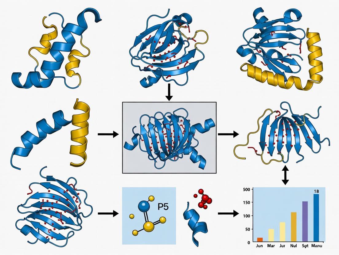
Striking evidence comes from de novo designed proteins. As shown in Table 1, a single point mutation (e.g., L45Y) in a 56-amino-acid chain can trigger a complete structural metamorphosis from a 3α helical fold to a 4β + α fold [15]. This dramatic shift, driven by a minimal sequence change, underscores that the hydrophobic core is not a passive container but a dynamically determined system. The folding pathway and final architecture are a synergistic outcome, where a single mutation can alter the collective interactions of all residues, leading to the construction of a completely different hydrophobic core [15].
Table 1: Impact of Single Mutations on Protein Core Structure and Global Fold in De Novo Proteins
| Protein Name | PDB ID | Mutation(s) | Chain Length | Resulting Structural Form | Core Implication |
|---|---|---|---|---|---|
| Ga98 | 2LHC | None | 56 aa | 3α | Reference hydrophobic core |
| Gb98 | 2LHD | L45Y | 56 aa | 4β + α | Single mutation triggers alternative core and fold |
| Gb98-T25I | 2LHG | L45Y, T25I | 56 aa | 3α | Compensatory mutation restores original core/fold |
| Gb98-T25I,L20A | 2LHE | L45Y, T25I, L20A | 56 aa | 4β + α | Additional mutation again switches core/fold |
Relative Contribution of Hydrophobic vs. Polar Interactions
The heterogeneity of the core also relates to the balance of different interaction types. While hydrophobic interactions are a primary contributor to thermodynamic stability, their role in mechanical stability is different. Steered molecular dynamics simulations reveal that when a protein is mechanically unfolded, the contribution of hydrophobic interactions to the resistance force is modest (one fifth to one third of the total force), while hydrogen bonds provide the majority of the mechanical resistance [10]. This contrast highlights a critical functional differentiation: the heterogeneous core is optimized not just for thermodynamic stability in the native state, but also for specific mechanical properties, with hydrogen bonds playing a disproportionately important role in resisting mechanical deformation [10].
Experimental Methodologies and Quantitative Analysis
Protocol: Quantifying Core Hydrophobicity with the FOD Model
The following is a detailed methodology for applying the FOD model to analyze a protein structure, as used in recent studies [14] [15].
- Data Acquisition: Obtain the three-dimensional atomic coordinates of the protein of interest from the Protein Data Bank (PDB).
- Theoretical Hydrophobicity Density (T) Calculation:
- Model the protein as a collection of atoms occupying discrete points in space.
- Define a theoretical hydrophobic density field, (\rhot(x, y, z)), using a 3D Gaussian function centered on the protein's geometric center: (\rhot(x, y, z) = \exp\left(-\frac{(x-x0)^2}{2\sigmax^2} - \frac{(y-y0)^2}{2\sigmay^2} - \frac{(z-z0)^2}{2\sigmaz^2}\right)) where (x0, y0, z0) are the coordinates of the center, and (\sigma) values define the spread of the distribution along each axis.
- Normalize the (\rhot) values so that the total sum of theoretical density across the entire protein volume equals 1.
- Empirical Hydrophobicity Density (O) Calculation:
- Assign an intrinsic hydrophobicity value to each amino acid residue in the chain (e.g., from a standardized scale like the Kyte-Doolittle scale).
- Smear this hydrophobicity value over the space occupied by the residue, typically using a Gaussian function centered on the residue's representative atom (e.g., Cα). This generates an empirical density field, (\rhoo(x, y, z)).
- Normalize the (\rhoo) values so that its total sum also equals 1.
- Divergence Calculation:
- Quantify the discrepancy between the theoretical (T) and observed (O) distributions using the Kullback-Leibler divergence: (D{KL}(O||T) = \sumi Oi \log\left(\frac{Oi}{Ti}\right)) where the sum is over all individual grid points (i) in the volume.
- A lower (D{KL}) value indicates a hydrophobic core that is closer to the idealized Gaussian model, while a higher value signifies greater disorder or heterogeneity.
- Analysis: Interpret the results in a biological context. A high divergence value may indicate a protein with a heterogeneous core, potentially prone to conformational changes, ligand binding, or aggregation, as seen in amyloidogenic proteins [14].
Protocol: Simulating Mechanical Unfolding via Steered Molecular Dynamics
This protocol is used to deconstruct the contribution of different interactions within the core to mechanical stability [10].
- System Preparation:
- Obtain the protein's PDB structure. Place it in a simulation box filled with explicit water molecules (e.g., TIP3P model).
- Add ions (e.g., Na⁺, Cl⁻) to neutralize the system's charge and achieve a physiologically relevant ionic concentration.
- Energy Minimization and Equilibration:
- Perform energy minimization (e.g., using steepest descent algorithm) to remove any steric clashes.
- Run an equilibration molecular dynamics (MD) simulation under NVT (constant Number of particles, Volume, and Temperature) and NPT (constant Number of particles, Pressure, and Temperature) ensembles for hundreds of picoseconds to stabilize the system.
- Steered MD (SMD) Simulation:
- Select two atoms (e.g., the N-terminus and C-terminus) as pulling points.
- Apply a constant velocity pulling force to one atom while restraining the other, effectively stretching the protein. Alternatively, use a constant force protocol.
- Run the SMD simulation for several nanoseconds, recording the positions of all atoms over time.
- Force-Extraction Curve and Interaction Analysis:
- Plot the force exerted on the pulling atom against the extension of the protein to generate a force-extension curve.
- Monitor the rupture events of specific interactions (hydrogen bonds and hydrophobic contacts) by tracking distances between key atoms over time.
- Correlate peaks in the force-extension curve with the simultaneous unraveling of specific interaction types to attribute force contributions.
- Quantification: Calculate the relative contribution of hydrophobic interactions by integrating the force peaks attributed to hydrophobic surface unraveling and comparing it to the total integrated force. Studies using this method have found the hydrophobic contribution to be between 20% and 33% of the total force, with hydrogen bonds being the dominant contributor to mechanical resistance [10].
Quantitative Benchmarks from Structural Bioinformatics
Large-scale comparative analyses, such as those evaluating AlphaFold2 (AF2) predictions against experimental structures, provide indirect but powerful insights into core heterogeneity. AF2 achieves high accuracy in predicting stable, ground-state conformations with proper stereochemistry. However, it shows systematic limitations in capturing the full spectrum of biologically relevant states, particularly in flexible regions and ligand-binding pockets [16].
Table 2: AlphaFold2 Performance Metrics Revealing Limitations in Modeling Heterogeneous Cores
| Analysis Parameter | Finding | Implication for Protein Cores |
|---|---|---|
| Domain Variability | Ligand-binding domains (LBDs) show higher structural variability (CV=29.3%) than DNA-binding domains (CV=17.7%) [16]. | Cores in LBDs are more flexible and context-dependent, defying a single, static oil-drop model. |
| Ligand-Binding Pockets | AF2 systematically underestimates ligand-binding pocket volumes by 8.4% on average [16]. | The precise chemistry and packing of core residues around ligands are difficult to predict from sequence alone, highlighting subtle heterogeneity. |
| Conformational States | AF2 captures only single conformational states in homodimeric receptors where experimental structures show functionally important asymmetry [16]. | Protein cores can adopt different, functionally relevant conformations in identical subunits, a level of heterogeneity not captured by static models. |
Visualization of Concepts and Workflows
Protein Folding Model Evolution
This diagram illustrates the conceptual evolution from the classical oil drop model to the modern fuzzy oil drop and heterogeneous core models.
Hydrophobic Core Analysis Workflow
This workflow outlines the key steps for the computational analysis of a protein's hydrophobic core using the FOD model.
Table 3: Key Research Reagent Solutions for Studying Protein Cores
| Reagent / Resource | Function / Application | Specific Example / Note |
|---|---|---|
| Protein Data Bank (PDB) | Primary repository for experimentally determined 3D protein structures used for analysis and validation. | As of Jan 2025, contains >230,000 structures [16]. Essential for FOD model input. |
| De Novo Designed Proteins | Model systems with minimal sequence differences to study the direct impact of mutations on core formation and fold. | Proteins like Ga98/Gb98 (PDB: 2LHC, 2LHD) reveal metamorphosis via single mutations [15]. |
| AlphaFold2 Database | Source of AI-predicted protein structures for proteins lacking experimental data; benchmark for core variability. | Useful but may underestimate pocket volumes and miss conformational diversity in cores [16]. |
| Molecular Dynamics Software | Simulates protein dynamics and forced unfolding to quantify interaction contributions (e.g., GROMACS, NAMD). | Used in steered MD to show hydrophobic forces contribute 20-33% of mechanical resistance [10]. |
| Hydrophobicity Scales | Standardized values assigning hydrophobicity to each amino acid for empirical density calculation. | e.g., Kyte-Doolittle scale, used in step 3 of the FOD protocol [14] [15]. |
The evidence is clear: the classical oil drop model, while historically valuable, is insufficient to describe the sophisticated reality of protein cores. The core is a heterogeneous, chemically diverse environment whose structure emerges from the synergistic collaboration of the entire polypeptide chain, sensitive to minimal sequence changes and yielding diverse mechanical and thermodynamic properties. The adoption of the fuzzy oil drop model and the study of metamorphic proteins provide the conceptual and quantitative frameworks to understand this heterogeneity. Furthermore, the limitations of powerful AI prediction tools like AlphaFold2 in capturing the full conformational spectrum of binding pockets and flexible domains serve as a critical reminder that the heterogeneous chemistry of the core is a central challenge in computational structural biology [16]. For researchers and drug development professionals, embracing this complexity is paramount. It opens new avenues for structure-based drug design by targeting specific, alternative core conformations, and for understanding the fundamental mechanisms of protein misfolding diseases, where the failure to form a correct, heterogeneous core leads to pathological aggregation.
The role of water in biological processes extends far beyond that of a passive solvent. In phenomena ranging from protein folding to molecular recognition, water acts as an active participant whose properties and behaviors fundamentally dictate thermodynamic outcomes. The theoretical construct known as the hydrophobic effect provides the primary framework for rationalizing how water molecules stabilize the folded state of proteins and facilitate other essential biological processes [17]. This whitepaper examines the molecular mechanisms through which water influences biomolecular folding and stability, with a specific focus on three interconnected concepts: the historical clathrate cage model, the modern understanding of solvent entropy, and the statistical mechanical perspective of cavity creation.
The classic explanation, heavily influenced by Kauzmann's 1959 review, posited that nonpolar side chains cluster together to form a nonpolar core, resembling an organic liquid—the so-called "oil drop model" of protein folding [17]. This view attributed the driving force for hydrophobic association to the entropy gain resulting from the release of ordered water molecules that formed structured "icebergs" or clathrate-like cages around nonpolar solutes. However, advancing research in statistical mechanics and computational modeling has challenged aspects of this traditional view, leading to a more nuanced understanding of how water actively participates in and drives biomolecular organization.
Theoretical Frameworks: From Clathrate Cages to Cavity Creation
The Traditional Clathrate Cage Model
The classic Kauzmann explanation of the hydrophobic effect emerged from observations that the Gibbs free energy change of transfer for hydrocarbon species from organic liquids to water is largely positive and entropy-dominated [17]. This entropy dominance was historically attributed to water's purported ability to form ordered three-dimensional structures—often described as "icebergs" or clathrate cages—around nonpolar species that cannot participate in hydrogen bonding with the solvent network. According to this model, when nonpolar groups associate in water, these structured water molecules are released back into the bulk solvent, gaining translational entropy and thereby providing the thermodynamic driving force for hydrophobic interactions.
However, this traditional view faces several theoretical and experimental challenges. The existence of such extensively ordered structures around nonpolar solutes has never been conclusively demonstrated in liquid water at physiological temperatures [17]. The clathrate cage model represents an appealing but potentially oversimplified conceptualization of what occurs at the molecular level when water interacts with nonpolar surfaces.
Modern Statistical Mechanical Perspective
Contemporary statistical mechanical analysis provides an alternative framework for understanding hydrophobic hydration. According to this perspective, the key concept is cavity creation—the theoretical process of creating a void space in water at a fixed position to host a solute molecule [17]. This construct accounts for the fundamental physical fact that all molecules possess volume and cannot occupy the same space simultaneously.
The process of cavity creation in water carries a significant Gibbs free energy cost (ΔGc) that increases with the liquid's number density [17]. Water, with its exceptionally high number density due to small molecular size, therefore imposes a substantial thermodynamic penalty for cavity creation. The presence of a cavity generates a solvent-excluded volume effect that affects all surrounding water molecules as they undergo continuous translational motion. This exclusion effect reduces the translational entropy of water molecules by restricting their accessible configurational space—a phenomenon particularly pronounced in water due to its high number density.
Table 1: Comparison of Historical and Modern Views of the Hydrophobic Effect
| Aspect | Traditional View (Clathrate Cages) | Modern View (Cavity Creation) |
|---|---|---|
| Driving Force | Release of structured water molecules | Gain in translational entropy of water |
| Molecular Origin | Hydrogen bond reorganization | Excluded volume effects |
| Water Structure | Iceberg-like clusters around nonpolar groups | Liquid water with restricted configurations |
| Entropy Dominance | Due to melting of ordered structures | Due to increased translational freedom |
| Theoretical Basis | Analogous to clathrate compounds | Statistical mechanics of dense liquids |
When a protein folds, the reduction in water-accessible surface area (WASA) reduces the total excluded volume effect, allowing more configurational space for water molecules and thereby increasing their translational entropy [17]. This entropy gain represents the fundamental driving force behind protein folding from the solvent's perspective. The modern view thus maintains that "the gain in translational entropy of water molecules (due to the decrease in water-accessible surface area associated with folding) is the driving force behind protein folding" [17], but through the mechanism of reduced excluded volume rather than the breakdown of clathrate-like structures.
Computational Methodologies for Investigating Hydration
Molecular Dynamics Simulations
Molecular Dynamics (MD) simulations have become indispensable tools for studying the behavior of water in biological systems at atomic resolution. MD is a computational technique that evaluates a molecular system's thermodynamic properties and conformational behavior over time by numerically solving Newton's equations of motion for all atoms in the system [18] [19]. In the context of protein folding and hydration, MD simulations typically employ an atomistic "all-atom" approach where the model system consists of a collection of interacting particles represented as atoms, describing both the solute biomolecule and the surrounding solvent water molecules [19].
Modern MD simulations of biomolecular systems are generally performed using the following protocol [18] [20]:
- System Preparation: The protein structure from experimental data is solvated in a water box, with ions added to achieve physiological concentration and neutrality.
- Force Field Selection: Empirical potential energy functions are applied to describe atomic interactions.
- Energy Minimization: The system is relaxed to remove steric clashes.
- Equilibration: The system is gradually brought to the target temperature and pressure.
- Production Run: The final trajectory is generated for analysis.
For proteins, simulations are typically conducted in the isothermal-isobaric (NPT) ensemble using software packages such as GROMACS, AMBER, or NAMD [19] [20]. The GROMOS 54a7 force field is commonly employed for modeling biomolecules, with water represented by models such as TIP3P, TIP4P, or SPC [20]. Simulation boxes are typically cubic with periodic boundary conditions applied to minimize edge effects, with system sizes ranging from tens of thousands to millions of atoms depending on the biological question [19].
Grid Inhomogeneous Solvation Theory
Grid Inhomogeneous Solvation Theory provides a powerful methodological framework for analyzing water structure and thermodynamics from MD trajectories. GIST discretizes the analytical expressions of inhomogeneous solvation theory onto a spatial grid, allowing calculation of thermodynamic quantities at each voxel throughout the system [21].
The key equations underlying GIST analysis are:
The solvation free energy: ΔGₛₒₗᵥ = ΔEₛₒₗᵥ - TΔSₛₒₗᵥ [21]
The solvation enthalpy: ΔEₛₒₗᵥ = ΔEₛᵥ + ΔEᵥᵥ [21]
The solvation entropy: ΔSₛₒₗᵥ = ΔSₜᵣₐₙₛ + ΔSₒᵣᵢₑₙₜ [21]
Where ΔEₛᵥ represents solute-water interactions, ΔEᵥᵥ represents water-water interactions, ΔSₜᵣₐₙₛ represents translational entropy, and ΔSₒᵣᵢₑₙₜ represents orientational entropy. This decomposition enables researchers to separately quantify the enthalpic and entropic contributions to hydrophobicity, providing unprecedented insight into the molecular origins of hydrophobic effects [21].
Table 2: Key Properties Calculated from MD Simulations for Hydration Analysis
| Property | Symbol | Description | Significance |
|---|---|---|---|
| Solvation Free Energy | ΔGₛₒₗᵥ | Free energy change for transferring solute from gas to water | Measures overall hydrophobicity |
| Solvent Accessible Surface Area | SASA | Surface area accessible to water molecules | Correlates with hydrophobic effect strength |
| Coulombic Energy | - | Electrostatic solute-solvent interactions | Measures polar contributions to solvation |
| Lennard-Jones Energy | LJ | van der Waals solute-solvent interactions | Measures nonpolar contributions |
| Translational Entropy | ΔSₜᵣₐₙₛ | Entropy from water position distribution | Key driver of hydrophobic effect |
| Orientational Entropy | ΔSₒᵣᵢₑₙₜ | Entropy from water orientation distribution | Measures ordering of water molecules |
Experimental Evidence and Case Studies
Water in Protein Folding and Stability
The role of water as an active participant in protein folding finds support in computational studies of specific protein systems. Research on the Peroxisome Proliferator-Activated Receptor γ provides a compelling case study. PPARγ is a nuclear receptor with a large, flexible active site characterized by a distinctive ω-loop that confers exceptional flexibility [18]. MD simulations of PPARγ complexed with Rosiglitazone (an anti-diabetic drug) revealed significant flexibility in the ω-loop region, with root mean square fluctuation values between 4-6 Å [18].
When Oleic Acid was introduced as a co-ligand binding to an alternate site, it produced a notable stabilization of the ω-loop, reducing RMSF values to 2-3 Å [18]. This stabilization occurred through allosteric modulation mediated by changes in the hydration environment. HINT-based analysis of the MD trajectories demonstrated that the binding event altered the intramolecular interactions between the flexible ω-loop and helix H3, with water molecules playing a crucial role in transmitting these allosteric effects [18].
Cavitation in Protein-Protein Interactions
Cavitation—the formation of vapor-filled cavities in liquids when pressure falls below the vapor pressure—represents an extreme manifestation of hydrophobic effects with significant implications for protein interactions [22]. In fluid mechanics and engineering, cavitation occurs when the static pressure of a liquid reduces to below the liquid's vapor pressure, leading to the formation of small vapor-filled cavities that collapse violently when subjected to higher pressure, generating shock waves [22].
In biological systems, cavitation phenomena can occur between hydrophobic protein surfaces. Studies of the melittin dimer system have provided direct observation of solvent-mediated hydrophobic protein-protein interactions [23]. When two melittin dimers associate through their hydrophobic contact regions, cavitation can occur between these surfaces. This cavitation was observed even with native electrostatic interactions intact [23]. Subsequent mutations that altered the geometry of the tetramer interface eliminated cavitation, demonstrating the exquisite sensitivity of this phenomenon to surface topography and chemical heterogeneity.
The process of cavitation between hydrophobic surfaces follows a predictable pattern: "When one turns to the molecular details of the mechanism of nonpolar aggregation in water, the picture is still not completely clear. The two limiting scenarios for events such as protein folding and directed self-assembly are [...] In the traditional view, water is gradually reduced within and between the associating regions in a manner that is concerted with their spatial approach. In an alternative cavitation scenario, a thermodynamic instability leads to water evacuation from the intervening space between hydrophobic regions, and the 'hydrophobic collapse' to contact then follows; the processes are sequential." [23]
Hydrophobicity Scales and Their Limitations
Traditional hydrophobicity scales assign a value to each amino acid describing its relative hydrophobic character. While useful for predicting protein secondary structures, membrane regions, and interior-exterior distributions, these scales have significant limitations [21]. They represent averaged hydrophobic character over entire amino acids, lacking spatial resolution to identify heterogeneous regions within binding pockets. Furthermore, conventional scales cannot directly measure entropic contributions to hydration, instead estimating them indirectly from temperature dependence of free energy or as the difference between free energy and enthalpy [21].
Advanced computational approaches now enable more sophisticated characterization of hydrophobicity. Methods combining MD simulations with GIST analysis can directly calculate entropic contributions from the phase space occupied by water molecules, providing both spatial resolution and separation of enthalpic and entropic components [21]. This represents a significant advancement over traditional hydrophobicity scales and offers new insights into the true nature of hydrophobic hydration.
Practical Implications in Drug Discovery and Development
Solubility Prediction and Optimization
Understanding water-solute interactions has direct applications in predicting and optimizing drug solubility—a critical factor in pharmaceutical development. Machine learning analysis of MD-derived properties has identified key descriptors correlating with aqueous solubility, including logP (octanol-water partition coefficient), SASA, Coulombic interactions, Lennard-Jones interactions, estimated solvation free energies, and structural fluctuation parameters [20].
These MD-derived properties demonstrate comparable predictive power for solubility to traditional structural descriptors, with gradient boosting algorithms achieving a predictive R² of 0.87 and RMSE of 0.537 [20]. This integration of MD simulations with machine learning represents a powerful approach for prioritizing compounds with optimal solubility profiles early in drug discovery, potentially reducing resource consumption and improving clinical success rates.
Protein Aggregation in Biopharmaceuticals
The role of water in protein stability has crucial implications for biopharmaceutical development, particularly regarding protein aggregation. Studies have revealed a synergistic effect between cavitation and agitation stresses in promoting antibody aggregation [24]. When vials containing protein solutions are subjected to dropping and shaking stresses—as may occur during shipping—cavitation bubbles form and collapse, generating extremely high local temperatures and pressures that can denature proteins [24].
The aggregation pathway induced by these combined stresses involves cavitation-induced unfolding followed by adsorption of unfolded antibodies to the container interface, then shaking-induced desorption of these adsorbed molecules, ultimately leading to particle formation [24]. This understanding informs stabilization strategies, such as adding nonionic surfactants like polysorbate 80, which lowers surface tension and prevents protein adsorption to interfaces [24].
Table 3: Research Reagents and Computational Tools for Hydration Studies
| Tool/Reagent | Type | Function/Application |
|---|---|---|
| GROMACS | Software | Molecular dynamics simulation package |
| AMBER | Software | Molecular dynamics simulation and force field |
| GROMOS 54a7 | Force Field | Empirical potential for biomolecular simulations |
| TIP3P/TIP4P | Water Model | Molecular representation of water properties |
| HINT | Scoring Function | Quantifies hydrophobic and polar interactions |
| GIST | Analysis Method | Grid-based solvation thermodynamics |
| Polysorbate 80 | Surfactant | Prevents protein adsorption at interfaces |
| PPARγ-Rosiglitazone | Protein-Ligand System | Model for studying hydration in allosteric modulation |
Water's role as an active participant in biological processes extends far beyond that of a passive solvent. The evolution from the historical clathrate cage model to the modern understanding of cavity creation and solvent entropy represents significant advancement in our conceptual framework. The gain in translational entropy of water molecules, resulting from reduced water-accessible surface area during folding, provides the fundamental driving force for protein stabilization, though through excluded volume effects rather than the breakdown of hypothetical ordered structures.
Computational methodologies, particularly Molecular Dynamics simulations coupled with advanced analysis techniques like Grid Inhomogeneous Solvation Theory, have revolutionized our ability to probe these phenomena at atomic resolution. These approaches enable researchers to decompose the enthalpic and entropic contributions to hydrophobicity, revealing the intricate balance of forces that govern biomolecular folding and recognition.
The practical implications of these insights span from drug design to biopharmaceutical development, informing strategies to optimize solubility, stability, and formulation. As computational power continues to grow and methodologies refine further, our understanding of water's active role in biological systems will undoubtedly deepen, opening new avenues for therapeutic intervention and biomolecular engineering.
For decades, the dominant paradigm in protein folding has emphasized the hydrophobic effect as the primary driving force, with the burial of non-polar side chains considered the fundamental organizing principle. This view posits that proteins fold to sequester hydrophobic residues away from aqueous solvent, forming a stable hydrophobic core. However, emerging research challenges the exclusivity of this narrative, revealing that the complete picture of protein stability and folding kinetics is far more complex. A comprehensive reassessment now points to the critical, and perhaps dominant, contributions of the protein backbone and polar groups—elements largely overlooked in traditional hydrophobicity-centric models.
The limitations of a purely hydrophobic framework become apparent when considering that the hydrophobic effect alone cannot explain the precise structural specificity of the native state or the rapid kinetics of folding. Statistical mechanical analyses indicate that the forces on hydrophilic groups are generally stronger than those on hydrophobic groups, with the magnitude of force on assemblies of hydrophilic groups dependent on their ability to form direct hydrogen bonds [25]. Furthermore, advanced simulation studies quantifying contributions to mechanical stability reveal that hydrophobic interactions account for only one-fifth to one-third of the total resistance to unfolding, with the remainder attributed primarily to hydrogen bonds [10]. This paper synthesizes recent experimental and computational evidence to establish a more balanced model of protein folding that fully incorporates the essential roles of the backbone and polar interactions.
Theoretical Foundation: Re-evaluating the Forces in Protein Folding
Statistical Mechanical Formalism of Folding Forces
A rigorous statistical mechanical framework helps clarify the distinct contributions to protein folding. The total potential of mean force (PMF) or free energy governing folding arises from both direct interatomic forces within the protein and solvent-induced forces. For a protein with configuration RM in a solvent of N water molecules with configuration XN, the partition function of the system is:
[ Q(T,V,N_T;R^M) = C \int e^{-\beta U(R^M,X^N)} dX^N ]
where ( \beta = (k_BT)^{-1} ), and ( U(R^M,X^N) ) represents the total potential energy of the system [25]. The thermodynamic force on any specific group i of the protein is then defined as the gradient of the Helmholtz energy with respect to positional changes of that group:
[ F(Ri) = -\nablai A(T,V,NT;R^M) = \frac{\int e^{-\beta U(R^M,X^N)} [-\nablai U(R^M,X^N)] dX^N}{\int e^{-\beta U(R^M,X^N)} dX^N} ]
This formalism separates forces into two categories: direct forces arising from interactions with other protein atoms, and solvent-induced forces arising from interactions with water molecules. Analysis of these components reveals that hydrophilic groups (HϕI) generally experience stronger forces than hydrophobic groups (HϕO), with the magnitude of force on HϕI assemblies being particularly dependent on their orientation and capacity to form hydrogen bonds [25].
The Hydrogen Bond Inventory Fallacy
The historical underestimation of polar contributions stems partly from the flawed "hydrogen bond inventory" argument, which suggested that intra-protein hydrogen bonds contribute minimally to stability because similar bonds could form with water in the unfolded state [25]. This perspective neglected the fundamental cooperativity of hydrogen bonding in proteins and the precise geometric alignment possible in the native state. Current estimates indicate that an intra-protein hydrogen bond can contribute up to 1.5 kcal/mol to stability, significantly more than previously thought [25].
Table 1: Quantitative Contributions of Different Interactions to Protein Stability
| Interaction Type | Estimated Energy Contribution | Primary Role in Folding |
|---|---|---|
| Intra-protein H-bond | Up to 1.5 kcal/mol [25] | Structural specificity, stability |
| Hydrophobic interaction | Variable, often <1 kcal/mol [25] | Global compaction, core formation |
| Protein-water H-bond | Contributes to net stability | Solvation, unfolded state destabilization |
| Electrostatic | Context-dependent | Directional stabilization, salt bridges |
Experimental Evidence: Quantitative Studies of Force Contributions
Mechanical Unfolding Simulations
Steered molecular dynamics simulations with constant-velocity pulling provide direct quantification of the forces resisting mechanical unfolding. These studies generate force-extension curves that reveal the distinct contribution patterns of different interaction types. For selected protein domains, hydrophobic forces account for only between one fifth and one third of the total force, with the remainder attributed primarily to hydrogen bonds [10].
A crucial finding is the different extension-dependency of these forces: hydrophobic force peaks shift toward larger protein extensions compared to force peaks from hydrogen bonds [10]. This indicates that hydrogen bonds provide early resistance to unfolding, while hydrophobic interactions persist longer during the extension process. The relative importance of hydrogen bonds over hydrophobic interactions in mechanical resistance contrasts with their traditional weighting in thermodynamic stability, highlighting the context-dependent nature of these contributions.
Water-Protein Hydrogen Bonding in Denatured States
Studies of the cold denatured state (CDS) and hot denatured state (HDS) of yeast frataxin provide additional insights into the role of hydration in protein stability. Research shows that water molecules in the bulk and at the protein interface form on average the same number of hydrogen bonds, with interface waters compensating for reduced water-water hydrogen bonds by forming additional protein-water hydrogen bonds [9].
At lower temperatures (272 K), where bulk water molecules form approximately 3.77 hydrogen bonds, the protein adapts by populating polyproline II conformations and becoming more expanded, allowing water to form approximately 83 additional hydrogen bonds with the protein that stabilize the cold denatured state [9]. In contrast, the hot denatured state (323 K) is more compact and richer in secondary structure, particularly α-helices, as water at higher temperatures forms fewer hydrogen bonds (approximately 3.55 per molecule) [9]. These structural adaptations demonstrate how proteins respond to maintain optimal hydrogen bonding with solvent across temperatures.
Table 2: Structural Properties of Cold vs. Hot Denatured States in Yeast Frataxin
| Property | Cold Denatured State (272 K) | Hot Denatured State (323 K) | Native State (298 K) |
|---|---|---|---|
| α-helical content | 6% | 10% | Higher than both denatured states |
| β-sheet content | 0.7% | 1.4% | Higher than both denatured states |
| Polyproline II content | 15% | 5% | Lower than denatured states |
| Radius of gyration | 1.7 nm | 1.6 nm | 1.5 nm |
| Average native contacts (Q) | 0.18 | 0.22 | 1.0 |
| Water H-bonds (bulk) | 3.77 | 3.55 | 3.66 |
Surface Hydrophobic Clusters in Coreless Proteins
The study of disintegrins—cysteine-rich proteins that lack a conventional hydrophobic core—provides exceptional insight into alternative stabilization strategies. These proteins maintain stability and solubility despite exposing hydrophobic residues on their surface through the formation of surface hydrophobic clusters (SHCs) [26].
SHCs are dynamic structural elements where exposed hydrophobic residues are protected by adjacent polar side chains and the shielding effect of protein solvation [26]. NMR CLEANEX experiments measuring water exchange rates (kex) of backbone amide hydrogens reveal that residues near SHCs exhibit higher local stability and protection from water exchange, while residues in the binding cleft show faster exchange with water and lower local stability [26]. This segregation of hydrophobic and solvent-permeable regions on opposite faces of the protein demonstrates how polar interactions and strategic solvation patterns can compensate for the absence of a traditional hydrophobic core.
Methodologies: Experimental Approaches for Studying Polar Contributions
NMR Characterization of Denatured States and Solvent Exchange
Restrained Molecular Dynamics with NMR Chemical Shifts
Purpose: To determine high-resolution structural ensembles of denatured states under various conditions [9].
Procedure:
- Acquire NMR chemical shift data for protein under denaturing conditions (e.g., 272 K for cold denaturation, 323 K for heat denaturation)
- Incorporate experimental chemical shifts as restraints in replica-averaged metadynamics (RAM) simulations
- Enhance conformational sampling through metadynamics while maintaining agreement with experimental data
- Analyze resulting structural ensembles for secondary structure content, radius of gyration, and solvent accessibility
- Calculate hydrogen bonding patterns for water molecules in bulk and at protein interface
Key Parameters: Chemical shift restraints, temperature conditions, simulation convergence criteria [9].
CLEANEX Experiments for Water Exchange Rates
Purpose: To identify protein regions with varying solvent accessibility and protection [26].
Procedure:
- Perform CLEANEX NMR experiments at multiple pH values (e.g., 6.0, 6.5, 7.0, 7.5)
- Measure water exchange rates (kex) of backbone amide hydrogens
- Map residues with fast exchange (kex > 1 s-1) versus protected residues
- Correlate exchange rates with structural features and stability measurements
- Identify surface hydrophobic clusters through segregation analysis of hydrophobic residues
Key Parameters: pH values, mixing times for CLEANEX, temperature, kex threshold for "fast exchange" [26].
Computational Approaches for Force Decomposition
Steered Molecular Dynamics with Constant-Velocity Pulling
Purpose: To decompose forces resisting mechanical unfolding into hydrophobic and hydrogen bonding contributions [10].
Procedure:
- Set up protein system with explicit solvent and appropriate force field
- Apply constant-velocity pulling to terminal residues
- Generate force-extension curves throughout unfolding trajectory
- Monitor hydrophobic surface exposure and hydrogen bond formation during extension
- Quantify force contributions by analyzing energy components and their spatial-temporal distribution
Key Parameters: Pulling velocity, force field parameters, solvation model, analysis methods for hydrophobic versus polar forces [10].
Φ-Value Analysis of Transition States
Purpose: To characterize differences in folding pathways under different conditions [9].
Procedure:
- Perform Φ-value analysis for both cold and hot denaturation processes
- Use Φ-values as restraints in molecular dynamics simulations
- Determine cold transition state (CTS) and hot transition state (HTS)
- Compare structural features of alternative transition states
- Correlate transition state differences with solvent hydrogen bonding capacity
The Scientist's Toolkit: Essential Research Reagents and Materials
Table 3: Key Research Reagents and Materials for Protein Folding Studies
| Reagent/Material | Function/Application | Specific Examples |
|---|---|---|
| Isotopically Labeled Compounds | NMR spectroscopy for structural studies | 15N- and 13C-labeled amino acids for protein expression [9] [26] |
| Chemical Denaturants | Protein unfolding studies, free energy calculations | Urea, guanidinium hydrochloride for denaturation curves [26] |
| Surfactants/Deter gents | Membrane protein studies, unfolding/refolding assays | Sodium dodecyl sulfate (SDS) for surfactant-induced unfolding [27] |
| Molecular Biology Tools | Protein expression and purification | Cloning vectors, expression systems for recombinant protein production |
| NMR Buffer Systems | Maintaining protein stability under varying conditions | pH buffers (e.g., phosphate, Tris) for CLEANEX experiments at multiple pH values [26] |
| Specialized Software | Data analysis, molecular dynamics simulations | Biotite for sequence analysis [28], Gecos for color scheme generation [29], Mol* for visualization [30] |
Implications for Drug Development and Protein Engineering
The revised understanding of protein folding forces has profound implications for pharmaceutical research and protein design. First, the critical role of polar interactions and backbone organization suggests new strategies for developing protein-based therapeutics. Stabilizing surface hydrophobic clusters through strategic introduction of polar residues could enhance stability without increasing aggregation propensity [26]. Second, drug design approaches can benefit from specifically targeting the more stable, water-protected regions of proteins rather than exclusively focusing on traditional hydrophobic pockets.
Furthermore, understanding the different mechanical behavior of hydrogen bonds versus hydrophobic interactions under extension [10] informs the design of mechano-resistant therapeutic proteins. Engineering strategies that enhance hydrogen bond networks at critical stress points could produce more robust protein therapeutics resistant to mechanical denaturation during production, storage, and delivery.
The evidence presented necessitates a fundamental shift in how we conceptualize the primary drivers of protein folding. While the hydrophobic effect remains an important contributor to global compaction and stability, the protein backbone and polar groups play equally critical, and in some contexts dominant, roles in determining folding pathways, structural specificity, and mechanical stability. The integrated model that emerges positions hydrogen bonding—both within the protein and with solvent water—as a central organizer of the native structure, with hydrophobic interactions providing additional stabilization particularly in the protein core.
This refined understanding resolves long-standing paradoxes in protein folding, including how proteins achieve such remarkable structural specificity and why folding occurs on biologically feasible timescales. The precise geometric requirements of hydrogen bonding and polar interactions provide the necessary directionality to guide efficient folding, complementing the more global driving force of hydrophobicity. As research in this area continues to evolve, further elucidating the intricate interplay between these forces will undoubtedly yield new insights into protein misfolding diseases, innovative therapeutic strategies, and novel biomaterials designed from first principles.
Quantifying and Applying Hydrophobicity in Protein Modeling and Design
Hydrophobicity, a fundamental physicochemical property, is a major driving force in protein folding, stability, and molecular recognition. This whitepaper surveys the evolution of hydrophobicity quantification, from early experimental scales based on solvent partitioning to modern computational and atomic-level approaches. We detail the theoretical underpinnings, methodological frameworks, and key applications of these scales, with a particular focus on their critical role in protein folding research and drug development. The integration of these scales into predictive computational models, such as the hydrophobic-polar (HP) model and all-atom simulations, has profoundly advanced our understanding of the hydrophobic effect, enabling more accurate prediction of protein structure and behavior. This guide provides researchers with a structured comparison of quantitative scales, detailed experimental protocols, and visualization of core concepts to inform the design and interpretation of studies in structural biology and biotherapeutics development.
The hydrophobic effect is widely recognized as one of the most important interactions in nature and a primary driving force in protein folding and stability [2]. This is predominantly an entropic phenomenon, originating from the disruption of the highly dynamic hydrogen-bond network of water by non-polar molecules. To minimize this disruption, water molecules form ordered "cages" or "icebergs" around non-polar moieties, resulting in a significant loss of entropy [2] [31]. The aggregation of non-polar molecules and the burial of hydrophobic residues in protein cores reduce the total hydrophobic surface area exposed to water, thereby increasing the system's overall entropy and making the process thermodynamically favorable [2].
The earliest studies connecting hydrophobicity to biological activity date back to Meyer and Overton, who correlated the hydrophobic nature of gases with their anesthetic potency [2]. Later, Kauzmann formalized the concept of the "hydrophobic bond" in protein folding, highlighting the tendency of non-polar side chains to associate in aqueous solutions [2] [32]. Although the term "bond" is somewhat misleading—as the interaction is primarily mediated by the solvent rather than a direct attraction—the core concept remains a cornerstone of structural biology [2]. Understanding and quantifying this effect is therefore paramount, leading to the development of numerous hydrophobicity scales that assign values to amino acids based on their relative hydrophobicity or hydrophilicity [31].
Experimental Hydrophobicity Scales
Experimental hydrophobicity scales are derived from empirical measurements of amino acid properties in various systems. These scales provide the foundational data for understanding residue-specific hydrophobic contributions.
Partition Coefficient-Based Scales (LogP)
The partition coefficient of a solute between water and a non-polar solvent, typically expressed as its logarithm (LogP), is a direct measure of hydrophobicity. The 1-octanol/water system (LogPo/w) became a standard due to its early adoption and relevance to biological systems [2]. Hansch and Leo's seminal 1971 work established a comprehensive framework for determining and using partition coefficients, demonstrating that the energy of partitioning per methylene group was approximately -690 cal mol⁻¹, a value that proved relevant to biological partitioning [2].
Core Protocol: Measuring Octanol-Water Partition Coefficients
- Preparation: Pre-saturate high-purity 1-octanol and water (or buffer) by mixing them thoroughly and allowing them to separate before use. This ensures neither phase alters the other during the experiment.
- Partitioning: Dissolve the solute (e.g., an amino acid derivative) in a known volume of one of the pre-saturated phases. Mix it with an equal volume of the other phase in a sealed container.
- Equilibration: Agitate the mixture vigorously at a constant temperature (e.g., 25°C) for a sufficient time to reach partitioning equilibrium.
- Separation and Analysis: Allow the phases to separate completely. Carefully separate the two phases and quantify the concentration of the solute in each phase using a suitable analytical method (e.g., UV spectroscopy, HPLC).
- Calculation: Calculate LogP using the formula: ( \text{LogP} = \log{10}(\frac{[C]{\text{octanol}}}{[C]_{\text{water}}}) ), where [C] is the equilibrium concentration in the respective phase.
Other Experimentally Derived Scales
Beyond solvent partitioning, several other methods have been developed, each with its own advantages and limitations.
Table 1: Methods for Deriving Experimental Hydrophobicity Scales
| Method | Description | Key Example(s) | Advantages | Limitations |
|---|---|---|---|---|
| Chromatographic Methods | Measures retention time on a non-polar stationary phase (e.g., Reversed-Phase Liquid Chromatography, RPLC). | [11] [31] | Effectively mimics biological membranes; suitable for peptides. | Results depend on parameters like silica surface area, buffer pH, and temperature. |
| Accessible Surface Area (ASA) Methods | Calculates the solvent-accessible surface area of amino acid residues within a protein and correlates it with hydrophobicity. | [32] [31] | Directly relates to the 3D structure of proteins. | Requires known 3D structures; the choice of empirical solvation parameters can influence results. |
| Site-Directed Mutagenesis | Measures the change in protein stability upon substituting a single amino acid. | [31] | Provides a direct, biologically relevant measure of protein stability. | Technically demanding, costly, and not all 20 amino acids can be easily substituted at a single site. |
| Physical Property Methods | Derives scales from physical properties like surface tension or heat capacity. | Scale based on surface tension measurements in NaCl solution [31]. | Experimentally straightforward and flexible. | Measurements (e.g., surface tension) may not fully capture the complexity of hydrogen-bond disruption. |
The Researcher's Toolkit: Essential Reagents and Materials
Table 2: Key Research Reagents for Hydrophobicity Studies
| Reagent/Material | Function in Experimentation |
|---|---|
| 1-Octanol | A model non-polar solvent used in the gold-standard LogP determination for partition coefficient studies [2]. |
| Sodium Dodecyl Sulfate (SDS) Micelles | Used as a model membrane system to measure the partitioning of amino acids, simulating a biological non-polar phase [31]. |
| C18-Bonded Silica Columns | The most common stationary phase in Reversed-Phase Liquid Chromatography (RPLC) for measuring peptide hydrophobicity [31]. |
| Urea/Guanidine Denaturants | Used in thermodynamic folding/unfolding experiments to measure protein stability and the contribution of hydrophobic interactions [25]. |
Computational Hydrophobicity Scales and Prediction Methods
Computational methods overcome many limitations of experimental scales by enabling high-throughput analysis and incorporating structural information.
Theoretical Estimation of LogP
Theoretical methods for predicting LogP can be broadly categorized as follows [2]:
- Fragment-Based Methods: These approaches, such as the methods by Rekker and the C-LOGP algorithm, decompose a molecule into fragments with known hydrophobic contributions. The overall LogP is summed from these fragments, with additive correction factors introduced to account for inter-fragmental interactions [2]. A criticism is that the fragmentation can be arbitrary.
- Atom-Based Methods: Methods like XLOGP and the Ghose-Crippen method assign hydrophobicity contributions to each atom type, reducing the reliance on predefined fragments and potentially offering more generalizability [2].
- Property-Based Approaches: Methods such as Toulmin's ΔLogP use molecular property descriptions to predict partitioning behavior [2].
Atomic-Level Hydrophobicity Scales
Residue-level scales treat an entire amino acid as a single value, which is problematic for amphiphilic residues containing both polar and non-polar atoms (e.g., tyrosine, lysine) [32]. To address this, atomic-level scales provide a more granular view. A prominent example is a simple binary atomic-level scale that classifies each atom as hydrophobic or hydrophilic based on its atom type in modern molecular mechanics force fields (e.g., CHARMM, AMBER) [32]. This approach accurately reflects the internal heterogeneity of amino acids and improves the visualization and quantification of protein surface hydrophobicity.
Structure-Based Hydrophobicity Scores
For folded proteins, structure-based methods often outperform sequence-based predictions. These methods incorporate the solvent-accessible surface area (SASA) to avoid contributions from the buried hydrophobic core. Key approaches include:
- Spatial Aggregation Propensity (SAP): Computes the sum of hydrophobicity values of surface-exposed side-chain atoms within a pre-defined cutoff radius, identifying hydrophobic patches on the protein surface [11].
- Hydrophobic Potentials: Maps hydrophobicity to the protein surface using a distance weighting function, favoring large contiguous hydrophobic patches over isolated hydrophobic atoms [11].
The following diagram illustrates the logical workflow for selecting and applying a hydrophobicity scale based on the research objective and available data.
Diagram 1: A decision workflow for selecting appropriate hydrophobicity scales and methods based on research objectives.
Application in Protein Folding: From Coarse-Grained to All-Atom Models
Hydrophobicity scales are integral to computational models that predict protein folding pathways and native structures.
The Hydrophobic-Polar (HP) Lattice Model
The HP model is a highly simplified but widely studied model for protein folding. It reduces the amino acid alphabet to two states: H (hydrophobic) and P (hydrophilic or polar) [33]. The protein chain is placed on a lattice (2D or 3D), and the goal is to find the configuration that maximizes the number of H-H contacts, which correspond to the lowest energy state [33] [34]. This model captures the essence of the hydrophobic driving force while being computationally tractable, though it is an NP-hard problem [33].
Advanced computational techniques have been employed to solve the HP model:
- Reinforcement Learning (RL): RL frameworks, such as Q-learning, structure the folding problem as a Markov decision process. The agent (the folding algorithm) learns to select actions (e.g., left, up, right, down on a 2D lattice) to maximize cumulative reward (based on energy minimization). RL with a full state space has been shown to robustly converge to the lowest energy conformations [33].
- Hybrid Algorithms: Methods like PSO-TS, which integrate Particle Swarm Optimization (PSO) with Tabu Search (TS), use PSO for global exploration and TS to avoid becoming trapped in local optima, providing highly accurate and stable predictions for both short and long sequences [34].
All-Atom Simulations and the Hydrophobic Effect
All-atom molecular dynamics (MD) simulations in explicit solvent provide the most detailed view of the hydrophobic effect. A key insight from such studies is that proteins, due to their complex surface patterns of polar and non-polar residues, can behave like "small" solutes (<1 nm) rather than "large" ones [9]. For small solutes, water can form hydrogen-bond networks around them, making the hydrophobic effect entropy-driven at room temperature. For large, flat hydrophobic surfaces, the water network is disrupted, leading to different scaling laws [9].
Studies comparing cold denatured states (CDS) and hot denatured states (HDS) reveal that the HDS is more compact and richer in secondary structure than the CDS. This is because water at lower temperatures can form more hydrogen bonds with the protein, stabilizing a more expanded CDS. In contrast, at higher temperatures, the drive to minimize the hydrophobic surface area dominates, leading to a more compact HDS [9]. This difference in solvent-protein interactions results in alternative folding transition states for cold versus hot denaturation [9].
The following diagram outlines a general computational workflow for predicting protein structure using hydrophobicity-driven models.
Diagram 2: A computational workflow for protein structure prediction leveraging hydrophobicity, from coarse-grained to all-atom models.
Comparative Analysis of Hydrophobicity Scales
The performance of a hydrophobicity scale is highly context-dependent. A scale that excels at predicting transmembrane helices may perform poorly in ranking antibody hydrophobicity for developability.
Table 3: Comparison of Selected Hydrophobicity Scales
| Scale Name | Type | Basis of Derivation | Key Amino Acid Rankings (High to Low Hydrophobicity) | Typical Application Context |
|---|---|---|---|---|
| Wimley-White Interfacial [31] | Whole Residue | Experimental transfer free energies of unfolded peptides from water to bilayer interface. | Trp (-1.85) > Phe (-1.13) > Leu (-0.56) > Ile (-0.31) > ... > Arg (≈0.81) | Predicting peptide partitioning into lipid bilayers; transmembrane helix identification. |
| Wimley-White Octanol [31] | Whole Residue | Experimental transfer free energies of unfolded peptides from water to n-octanol. | Trp (-2.09) > Phe (-1.71) > Leu (-1.25) > Ile (-1.12) > ... > Arg (≈0.81) | Modeling partitioning into hydrophobic cores; general protein stability. |
| Atomic-Level (Binary) [32] | Atomic | Classification of individual atoms as hydrophobic/non-polar or hydrophilic/polar based on force-field types. | N/A (Atom-based: e.g., aliphatic C is hydrophobic; O, N are hydrophilic). | Detailed visualization and quantification of protein surface hydrophobicity; analyzing binding interfaces. |
| Spatial Aggregation Propensity (SAP) [11] | Structure-Based | Computes local hydrophobicity density on the solvent-accessible surface of a folded protein. | Dependent on the underlying residue scale used and the 3D structure. | Identifying hydrophobic patches on antibodies and biotherapeutics to predict aggregation propensity. |
The journey from simple solvent partitioning experiments to sophisticated atomic-level and structure-based computational scales has profoundly expanded our understanding of the hydrophobic effect in protein folding. Each scale and model offers a unique lens: LogP and whole-residue scales provide a thermodynamic foundation for peptide behavior; the HP model captures the core driving force of folding in a computationally accessible way; and all-atom simulations reveal the critical role of water structure and dynamics. The choice of scale is paramount and must be dictated by the specific biological question, whether it is predicting transmembrane domains, optimizing antibody solubility, or simulating folding pathways.
Future research will likely focus on integrating these multi-faceted approaches. Machine learning models trained on diverse datasets that incorporate both experimental retention times and high-resolution structural features promise to generate more robust and universally applicable scales. Furthermore, as computational power increases, the use of explicit-solvent simulations to derive and validate hydrophobicity parameters will become more routine, bridging the gap between simplified models and biological reality. This continuous refinement of hydrophobicity quantification will remain central to unraveling the complexities of protein folding, stability, and function, ultimately accelerating rational drug design and protein engineering.
The prediction of protein structure from amino acid sequence represents a fundamental challenge in computational biology. The native structure of a protein is widely accepted to be the conformation with the lowest free energy, with the hydrophobic effect serving as a primary driving force for folding [35]. In globular proteins, this manifests as a hydrophobic core constituted by non-polar amino acids, while polar residues typically reside on the surface, thereby segregating non-polar residues from the aqueous solvent [35]. This organization minimizes disruptive interactions with water and achieves a state of low energy, maximizing stability.
However, a complete physical model must integrate more than just hydrophobicity. Steric repulsion between atoms and chain segments prevents unrealistic atomic overlaps and defines the compactness of the folded state. Furthermore, the protein is a polymeric chain with specific connectivity and constraints; the backbone's conformational flexibility and the restrictions imposed by peptide bonds are critical for determining plausible folds. The interplay of these forces—hydrophobic interactions, steric repulsion, and polymer constraints—forms the tripartite foundation upon which robust computational folding models are built. This integration is especially crucial as the field progresses from static structure prediction to understanding dynamic conformational states, a key frontier in the post-AlphaFold era [36].
Quantitative Frameworks for Hydrophobicity and Polymer Physics
The Burial Mode Model: A Unified Theoretical Framework
A compelling approach that integrates these three principles is the "Burial Mode Model" [7]. This model provides a quantitative, yet computationally efficient, framework for predicting residue burial and conformational fluctuations from sequence alone. Its energy function explicitly incorporates the key physical forces:
- Polymer Constraints: The model represents the protein as a linear chain of N residues. The connectivity and elasticity of the backbone are captured through a harmonic spring-like term between adjacent monomers, with a bond stiffness parameter (κ) that sets the chain's extensibility.
- Hydrophobic Effect: The tendency of each amino acid to be buried or exposed is modeled using a hydrophobicity scale. The hydrophobic contribution to the energy is formulated to reflect that the force driving a residue toward the core is stronger near the surface than in the already buried core.
- Steric Repulsion: A global constraint is imposed on the ratio (α) of the squared gyration radius to the squared maximum distance from the center of mass. This prevents an unrealistic collapse of all residues into the center, effectively accounting for the limited space in the protein core and enforcing proper packing.
For a typical 100–300 residue protein, this model can compute tertiary structural information in less than a second on a single CPU, making it suitable for large-scale analysis [7]. The model's output is an energy-minimizing "burial trace"—the predicted squared distance of each residue from the molecular center of mass—which can be directly compared to traces derived from experimental structures.
Hydrophobicity Scales and Parameter Optimization
The performance of physical models like the burial mode model depends on accurate parameterization. Hydrophobicity scales are particularly important, and they are generally derived through two main approaches [7]:
- Experimental Scales: Based on measurements of the free energy of solvation of amino acids or short peptides in different solvents (e.g., water, ethanol). The Kyte-Doolittle scale is a classic example.
- Numerical Scales: Derived from statistical analysis of the partitioning of amino acid residues between the core and surface in large datasets of known protein structures.
Optimization studies have revealed that classic hydrophobicity scales like Kyte-Doolittle are already nearly optimal for predicting residue burial in the burial mode model, though fine-tuning from structural data remains an active area of research [7].
Table 1: Key Physical Parameters in the Burial Mode Model
| Parameter | Physical Significance | Typical Value/Range |
|---|---|---|
| Bond Stiffness (κ) | Controls the elastic extensibility of the polypeptide chain; sets the unit of length. | Chosen so the mean-square distance between neighbors is 1. |
| Packing Parameter (α) | Constrains the protein's compactness, enforcing steric repulsion and limited core volume. | 0.4 - 0.6 (set to 3/5 for a uniform spherical globule). |
| Amino Acid Hydrophobicities | Determines the relative driving force for each residue type to be buried in the core or exposed to solvent. | Derived from experimental (e.g., Kyte-Doolittle) or numerical scales. |
| Maximum Radius (R_max) | The estimated physical radius of the folded protein domain, based on chain length. | ( R_{max} = (3N/(4\pi\rho))^{1/3} ), where (\rho) is monomer density. |
Experimental Protocols for Validating Physical Models
Protocol: Adversarial Testing for Physical Robustness
With the rise of deep learning co-folding models like AlphaFold3 and RoseTTAFold All-Atom, new protocols are needed to test whether these data-driven models have learned the underlying physics or are merely memorizing training data patterns [37]. The following adversarial testing protocol, based on recent research, serves this purpose.
1. Principle: Challenge the model with biologically plausible but physically disruptive perturbations. A model that understands physics should predict commensurate structural changes.
2. System Setup:
- Protein Target: Select a well-characterized protein-ligand complex (e.g., Cyclin-dependent kinase 2 (CDK2) with ATP).
- Computational Models: Subject the system to multiple state-of-the-art co-folding models (e.g., AlphaFold3, RoseTTAFold All-Atom, Chai-1, Boltz-1).
3. Experimental Challenges:
- Binding Site Removal: Mutate all binding site residues to glycine. This removes side-chain interactions without introducing steric clashes.
- Binding Site Occlusion: Mutate all binding site residues to bulky residues like phenylalanine. This removes favorable interactions and sterically occludes the original pocket.
- Chemical Property Inversion: Mutate binding site residues to residues with dissimilar chemical properties (e.g., positively charged to negatively charged), drastically altering the site's electrostatic landscape.
4. Data Analysis:
- Primary Metric: Calculate the Root-Mean-Square Deviation (RMSD) of the predicted ligand pose compared to the wild-type prediction and the known native structure.
- Qualitative Assessment: Visually inspect predictions for maintenance of physically unrealistic poses (e.g., ligand remaining in an occluded pocket) and the presence of steric clashes.
This protocol has revealed that some deep learning models continue to place ligands in original binding sites even after all native interactions have been removed, indicating a potential failure to generalize based on first principles [37].
Protocol: Analyzing Hydrogen Bonding in Denatured States
Understanding the role of the solvent and its interaction with the protein is crucial for a complete physical picture. This protocol characterizes the hydrophobic effect by analyzing the hydrogen-bonding networks in different denatured states [9].
1. Principle: The behavior of water molecules at the protein interface compared to the bulk reveals whether a protein's surface behaves like a "small" or "large" solute, which is fundamental to the hydrophobic effect.
2. System Setup:
- Protein Target: Use a protein whose cold and hot denatured states have been characterized experimentally (e.g., Yeast frataxin).
- Simulation Method: Employ Replica-Averaged Metadynamics (RAM) simulations, which use experimental NMR chemical shifts as restraints to achieve an atomic-resolution ensemble of structures for the denatured states.
3. Simulation and Analysis:
- State Generation: Perform RAM simulations under cold denaturation (CDS) and hot denaturation (HDS) conditions to generate structural ensembles.
- Hydrogen Bond Calculation: For each state, compute:
- The average number of hydrogen bonds per water molecule in the bulk.
- The average number of water-water and water-protein hydrogen bonds per water molecule in the first hydration shell (interface).
- Structural Metrics: Calculate the radius of gyration (Rg) and secondary structure content for the protein in each denatured state ensemble.
4. Key Insights:
- This protocol demonstrates that the total number of hydrogen bonds per water molecule is nearly identical in the bulk and at the protein interface, suggesting proteins behave like "small" solutes due to their complex surface patterns [9].
- It reveals that the cold denatured state is more expanded and has less secondary structure than the hot denatured state, as water at lower temperatures can form more hydrogen bonds, stabilizing a more expanded protein interface [9].
The Scientist's Toolkit: Research Reagent Solutions
Table 2: Essential Computational Tools and Models for Protein Folding Studies
| Tool/Reagent | Type | Primary Function |
|---|---|---|
| AlphaFold3 [37] | Deep Learning Model | End-to-end prediction of protein structures and complexes with ligands, nucleic acids, and other proteins. |
| RoseTTAFold All-Atom [37] | Deep Learning Model | Co-folding prediction of biomolecular complexes, similar to AlphaFold3. |
| Burial Mode Model [7] | Physics-Based Model | Rapid calculation of residue burial traces and conformational fluctuations from sequence using hydrophobicity and polymer physics. |
| Replica-Averaged Metadynamics (RAM) [9] | Simulation Method | Enhanced sampling molecular dynamics that incorporates experimental NMR chemical shifts as restraints to model denatured states and other conformers. |
| Chai-1 / Boltz-1 [37] | Deep Learning Model | Open-source co-folding models designed to achieve AlphaFold3-level accuracy. |
| AutoDock Vina [37] | Physics-Based Docking | Conventional molecular docking tool for predicting protein-ligand binding poses and affinities. |
| Kyte-Doolittle Hydropathy Scale [7] | Parameter Set | A standard hydrophobicity scale derived from experimental data, used to convert protein sequence into numerical values for physical models. |
Current Limitations and Future Directions
Despite significant advances, current computational models face notable challenges. The adversarial testing of deep learning co-folding models reveals critical limitations in their physical understanding. For instance, when binding site residues of CDK2 were mutated to glycine or phenylalanine, models like AlphaFold3 and RoseTTAFold All-Atom often continued to predict the ATP ligand in its original pose, despite the removal of favorable interactions or the introduction of severe steric clashes [37]. This indicates that these models can be overfit to specific data patterns in their training corpus and may lack robust generalization based on fundamental physics.
The future of the field lies in moving "beyond static structures" to model protein dynamics and multi-state conformations, which are fundamental to biological function [36]. This shift requires a deeper integration of physical principles with data-driven approaches. Combining the computational efficiency of models like the burial mode model with the accuracy of deep learning, and constraining both with high-quality experimental data from techniques like NMR, will be essential. Furthermore, improving the explicit handling of solvent effects, as demonstrated in the analysis of hot and cold denatured states, will lead to a more nuanced and predictive theory of the hydrophobic effect in protein folding and binding [9].
Visualizing Workflows and Relationships
Adv. Test Workflow
Folding Forces
Predicting Binding Sites and Fluctuations from Sequence Hydrophobicity Patterns
The hydrophobic effect is widely recognized as a primary driving force in protein folding and stability [38] [9] [8]. This fundamental phenomenon describes the tendency of nonpolar substances to aggregate in aqueous solutions, minimizing their contact with water molecules. In protein biochemistry, this effect manifests as the burial of hydrophobic amino acid side chains within the protein core, while polar and charged residues tend to occupy the solvent-exposed surface [39] [8]. This segregation maximizes entropy by minimizing the disruption of water's hydrogen-bonding network and represents a crucial determinant of three-dimensional protein structure.
Understanding and predicting protein structure and function from amino acid sequences remains a central challenge in molecular biology. The correlation between sequence hydrophobicity patterns and structural features provides a powerful approach for addressing this challenge. Hydrophobicity profiling enables researchers to identify potential receptor binding domains, predict protein flexibility, and elucidate molecular recognition mechanisms—insights with profound implications for drug design and therapeutic development. This technical guide explores the theoretical foundations, methodological approaches, and practical applications of hydrophobicity-based analysis for predicting binding sites and structural fluctuations in proteins.
Theoretical Foundations of the Hydrophobic Effect
Molecular Basis of Hydrophobic Interactions
The hydrophobic effect originates from the unique properties of water and its interaction with nonpolar solutes. When a nonpolar molecule or molecular region is introduced into water, the hydrogen-bonding network of water molecules reorganizes to form a structured "cage" or clathrate around the nonpolar surface. This restructuring leads to significant losses in translational and rotational entropy of water molecules, making the process thermodynamically unfavorable [8]. The free energy change associated with this process can be quantified as ΔG = ΔH - TΔS, where the entropic component (TΔS) dominates at room temperature.
Molecular dynamics simulations have quantified the hydrophobic effect by demonstrating that the free energy of cluster formation is proportional to the loss in exposed molecular surface area, with a constant of proportionality of 45 ± 6 cal/mol·Å² for molecular surface area, which corresponds to approximately 24 cal/mol·Å² for solvent-accessible surface area [40]. This linear relationship between hydrophobic interaction energy and burial of solvent-accessible surface area provides the physical basis for predicting protein folding and molecular recognition.
Hydrophobicity Scales and Their Applications
Various hydrophobicity scales have been developed to quantify the relative hydrophobicity of amino acids, employing different methodological approaches including water-vapor transfer free energies, statistical analysis of side-chain distributions in known protein structures, and theoretical calculations of transfer free energies [39]. The correlation between these hydrophobicity sequences and surface-exposure patterns in known protein structures, while statistically significant, is far from optimal, with mean correlation coefficients generally below 0.5 [39]. This imperfect correlation arises from several factors, including the high degree of mutational tolerance in naturally occurring proteins and the influence of forces beyond hydrophobicity in determining final protein structure.
Table 1: Commonly Used Hydrophobicity Scales and Their Characteristics
| Scale Name | Basis of Determination | Key Amino Acid Rankings | Applications |
|---|---|---|---|
| Kyte & Doolittle [39] | Water-vapor transfer free energies, side-chain distributions | Varies by method | General hydrophobicity profiling |
| Engelman et al. [39] | Transfer free energies for α-helical side chains | Nonpolar residues in transmembrane domains | Membrane protein prediction |
| Nozaki & Tanford [39] | Solubilities in water and ethanol relative to glycine | Based on experimental transfer energies | Solvation energy calculations |
| Miyazawa & Jernigan [39] | Residue-residue contact potentials | Statistically derived from known structures | Protein folding and docking |
Predicting Binding Domains from Hydrophobicity Profiles
Methodological Framework
The prediction of receptor binding domains using hydrophobicity profiles relies on calculating two key parameters: mean hydrophobicity and hydrophobic moment. Mean hydrophobicity measures the average hydrophobic character of a peptide segment, while hydrophobic moment quantifies the amphiphilicity or asymmetry in the spatial distribution of hydrophobic and hydrophilic residues along the protein chain [41]. These parameters are typically calculated using a sliding window approach across the protein sequence.
Experimental studies have validated this approach by demonstrating that receptor binding domains in apolipoprotein E correspond to regions with high hydrophilicity and high mean helical hydrophobic moment [41]. Specifically, two binding domains (residues 136-160 and 214-236) were identified in apolipoprotein E using this methodology, with the first domain subsequently confirmed experimentally. Mutations affecting hydrophobicity parameters in these regions significantly impact receptor binding affinity, confirming the functional importance of these predicted domains.
Protocol: Binding Site Prediction Using Hydrophobicity Profiling
Sequence Preparation: Obtain the protein amino acid sequence in FASTA format. Ensure sequence accuracy and completeness.
Hydrophobicity Scale Selection: Choose an appropriate hydrophobicity scale based on your specific application (see Table 1). The Kyte-Doolittle scale is often used as a default for general applications.
Parameter Calculation:
- Apply a sliding window (typically 7-21 residues) to calculate mean hydrophobicity at each position
- Compute hydrophobic moment using the formula: μH = √[(ΣHₙsin(δn))² + (ΣHₙcos(δn))²], where Hₙ is the hydrophobicity of residue n, and δ is the angle (typically 100° for α-helices)
- Generate profiles plotting these parameters against sequence position
Domain Identification:
- Identify regions with high hydrophilicity (low mean hydrophobicity) combined with high hydrophobic moment
- Rank potential binding domains based on these combined criteria
- Compare with known structural features (if available) for validation
Experimental Verification:
- Design peptides corresponding to predicted domains
- Assess binding affinity using surface plasmon resonance, isothermal titration calorimetry, or competitive binding assays
- Validate functional significance through site-directed mutagenesis of key residues
Figure 1: Workflow for predicting binding sites from sequence hydrophobicity patterns
Predicting Structural Fluctuations from Hydrophobicity Patterns
Residue-Specific Fluctuation Propensities
Protein residues exhibit characteristic fluctuation patterns based on their physicochemical properties and structural context. Analysis of normalized equilibrium fluctuations of residue centers of mass has enabled classification of amino acids into three distinct mobility groups [42]:
Table 2: Amino Acid Classification by Fluctuation Propensity
| Fluctuation Group | Mobility Ratio | Amino Acids | Structural Preferences |
|---|---|---|---|
| Highly fluctuating | >1.0 | Gly, Ala, Ser, Pro, Asp | Loops, disordered regions |
| Moderately fluctuating | 0.7-1.0 | Thr, Glu, Asn, Lys, Cys, Gln, Arg, Val | Mixed preferences |
| Weakly fluctuating | <0.7 | His, Leu, Met, Ile, Tyr, Phe, Trp | Regular secondary structures |
This classification reveals that highly fluctuating residues (Group I) show strong preferences for loop regions and disordered fragments, while weakly fluctuating residues (Group III) preferentially populate regular secondary structure elements (α-helices and β-strands) [42]. The correlation between fluctuation propensity and structural context provides a foundation for predicting protein flexibility directly from sequence information.
Protocol: Predicting Residue Fluctuation Profiles
Sequence Analysis:
- Identify amino acid types and their positions in the sequence
- Classify each residue according to its fluctuation group (Table 2)
Secondary Structure Prediction:
- Utilize tools like PSIPRED or Jpred to predict secondary structure elements
- Correlate fluctuation propensity with predicted secondary structure
Mobility Calculation:
- Apply normal mode analysis or elastic network models (e.g., Vibe program)
- Calculate mobility ratio for each residue: Rk = ⟨r₂k⟩/(r₂av), where ⟨r₂k⟩ is the mean square fluctuation of residue k, and r₂av is the average fluctuation of all residues [42]
Flexibility Mapping:
- Generate residue-wise flexibility profiles
- Identify regions of high and low flexibility
- Correlate flexibility patterns with potential functional sites
Thermostability Engineering:
- Identify highly fluctuating residues in critical regions
- Design mutations replacing highly fluctuating residues with weakly fluctuating ones
- Prioritize polar and charged weakly fluctuating residues for surface positions
Experimental Validation Techniques
Molecular Dynamics Simulations
Molecular dynamics (MD) simulations provide a powerful approach for validating predictions derived from hydrophobicity analysis. The following protocol outlines the key steps for quantifying hydrophobic interactions through MD simulations [40]:
System Setup:
- Select solute molecules (methane, butane, isobutylene, benzene)
- Create water-filled boxes of different sizes (e.g., 216 to 1,726 water molecules)
- Implement periodic boundary conditions
Simulation Parameters:
- Use NVE ensemble (constant number of molecules, volume, and energy)
- Set temperature to 298 K
- Utilize 2-fs time step for 1-ns simulation duration
- Employ fully flexible three-centered water model and all-atom solute representations
Cluster Analysis:
- Determine solute clusters using Voronoi polyhedron method
- Calculate molecular surface areas (total, solvent-exposed, and buried)
- Analyze cluster size distributions over trajectory
Free Energy Calculation:
- Compute free energy directly from distribution of cluster sizes
- Determine equilibrium constants for sequential solute addition
Binding Affinity Measurements
Fluorescence fluctuation experiments provide a robust method for quantifying ligand-protein binding equilibria [43]. The experimental protocol involves:
Sample Preparation:
- Titrate fluorescent ligands with protein
- Control buffer conditions to maintain physiological relevance
Data Collection:
- Measure fluctuation amplitude g(0) across titration series
- Record fluorescence intensity simultaneously
Data Analysis:
- Fit g(0) to binding model to determine dissociation coefficient
- Calculate number of binding sites
- Identify potential molecular heterogeneity in hapten-antibody complexes
Validation:
- Confirm molecular heterogeneity through fluorescence lifetime experiments
- Compare fractional populations and molecular brightness values
Table 3: Key Research Reagents and Computational Tools for Hydrophobicity Analysis
| Resource Type | Specific Examples | Function/Application |
|---|---|---|
| Computational Tools | BSpred [44] | Neural network-based binding site prediction from sequence |
| Simulation Software | ENCAD [40] | Molecular dynamics simulations with explicit solvent |
| Analysis Programs | Vibe [42] | Coarse-grained normal mode analysis for fluctuation prediction |
| Hydrophobicity Scales | Kyte-Doolittle, Engelman et al. [39] | Quantifying residue-specific hydrophobicity values |
| Experimental Assays | Fluorescence fluctuation [43] | Measuring binding equilibria and molecular heterogeneity |
| Structural Databases | Protein Data Bank | Access to known structures for validation and comparison |
The analysis of sequence hydrophobicity patterns provides powerful insights into protein structure and function, enabling prediction of binding sites and fluctuation propensities directly from amino acid sequences. The methodologies outlined in this technical guide—from hydrophobicity profiling to molecular dynamics simulations—offer researchers a comprehensive toolkit for investigating the role of hydrophobic effect in protein folding and molecular recognition.
While significant progress has been made in quantifying and applying these principles, challenges remain in achieving optimal correlation between hydrophobicity patterns and structural features. Future advances will likely emerge from integrated approaches combining hydrophobicity analysis with other biophysical parameters, machine learning algorithms, and high-resolution experimental techniques. These developments will further enhance our ability to decipher the protein folding code and accelerate drug discovery efforts targeting protein-protein interactions.
The strategic exploitation of hydrophobic effects represents a pivotal frontier in modern drug discovery, particularly for targeting protein-protein interactions (PPIs) and developing small-molecule inhibitors. PPIs mediate virtually all cellular processes and have emerged as a promising class of therapeutic targets for their direct association with disease pathways. However, these interfaces present unique challenges for drug development due to their characteristically large, flat, and topologically complex surfaces, which differ fundamentally from traditional deep binding pockets favored by conventional small-molecule drugs [45] [46]. The hydrophobic effect, recognized as a major driving force in protein folding and biomolecular recognition, offers powerful solutions to these challenges but requires careful balancing to avoid poor pharmacokinetic properties [1] [9].
This technical guide examines recent advances in leveraging hydrophobicity for drug design, with particular emphasis on PPI-targeting peptides and small-molecule inhibitors. We present quantitative analyses of hydrophobic contributions to binding energetics, detailed experimental protocols for solubility-aware design approaches, and practical toolkits for researchers working at this interface of physical chemistry and pharmaceutical development. The content is framed within the broader context of protein folding research, drawing connections between fundamental hydrophobic phenomena and their therapeutic applications.
Theoretical Foundation: Hydrophobic Effects in Protein Folding and Recognition
Molecular Basis of Hydrophobic Interactions
The hydrophobic effect arises from the tendency of nonpolar molecules or molecular surfaces to associate in aqueous environments, primarily driven by water's propensity to maintain its hydrogen-bonding network [1]. When hydrophobic groups cluster together, they minimize the disruption to surrounding water molecules, resulting in a net entropic gain that drives the association. This effect exhibits size-dependent behavior: for small solutes (<1 nm), hydration free energy scales with volume, while for larger solutes (>1 nm), it scales with surface area [1] [9]. This distinction has profound implications for drug design, as it determines whether hydrophobic binding contributions will be distributed or localized.
The structural biology of the hydrophobic effect reveals that water molecules at protein interfaces maintain their hydrogen-bonding capacity through a combination of water-water and water-protein interactions. Research on yeast frataxin demonstrated that the total number of hydrogen bonds per water molecule remains relatively constant (within 1%) for both bulk water and interface water, though the proportion of water-protein hydrogen bonds increases at the interface [9]. This compensation mechanism ensures that hydrophobic association doesn't come at excessive hydrogen-bonding costs, facilitating favorable binding thermodynamics.
Quantitative Contributions to Molecular Stability
Table 1: Hydrophobic Contribution to Protein Stability and Interactions
| System | Hydrophobic Contribution | Experimental Method | Reference |
|---|---|---|---|
| Protein domains (mechanical stability) | 20-33% of total force | Steered molecular dynamics | [47] |
| Protein folding (small solutes, <1nm) | ΔG scales with volume | Thermodynamic measurements | [1] [9] |
| Protein folding (large solutes, >1nm) | ΔG scales with surface area | Thermodynamic measurements | [1] [9] |
| Trypsin-protein interactions | Primary role in HSA/BSA binding | Multiple spectroscopic methods | [48] |
Hydrophobic and polar interactions contribute differentially to various stability measures. While hydrophobic effects provide significant thermodynamic stability, their contribution to mechanical stability is more modest. Steered molecular dynamics simulations reveal that hydrophobic interactions account for approximately one-fifth to one-third of the total force resistance during protein unfolding, with hydrogen bonds providing the predominant mechanical stabilization [47]. This distinction highlights the context-dependent nature of hydrophobic contributions and underscores the importance of matching interaction types to therapeutic objectives.
Targeting Protein-Protein Interactions: Challenges and Strategies
Structural Characteristics of PPI Interfaces
PPIs represent particularly challenging drug targets due to their extensive interface areas (typically 1,000-4,000 Ų compared to ~500 Ų for conventional drug targets) and their characteristically flat, featureless topographies [45] [46]. These interfaces frequently lack the deep, well-defined pockets that readily accommodate traditional small-molecule drugs, necessitating alternative targeting strategies. Additionally, PPI interfaces often comprise discontinuous binding epitopes that merge residues from distant sequence regions upon folding, further complicating inhibitor design [46].
Analysis of successful PPI inhibitors reveals they frequently target hot spots—specific regions within the larger interface that contribute disproportionately to binding energy. These hot spots often correlate with clusters of hydrophobic residues, which when effectively engaged, can disrupt the entire protein-protein interaction despite covering only a fraction of the total interface area [46]. This phenomenon provides a rational basis for designing smaller inhibitors that target these critical regions rather than attempting to cover the entire interface.
Peptide-Based PPI Targeting Strategies
Peptides offer a promising modality for PPI inhibition due to their ability to mimic structural elements of protein interfaces while maintaining sufficient flexibility to adapt to flat binding surfaces. Recent advances have demonstrated that approximately 58 therapeutic peptides targeting PPIs were in clinical development as of 2021, with 13 in Phase 1, 26 in Phase 2, 15 in Phase 3, and 4 with New Drug Applications pending [45].
However, peptide therapeutics face significant challenges related to membrane permeability and bioavailability. A critical concern is that peptides designed for high affinity often contain excessive hydrophobic character, leading to poor solubility and aggregation propensity. The "binder hallucination" protocol in AfDesign, for instance, tends to generate sequences with overrepresented aromatic and hydrophobic residues at interaction surfaces, resulting in undesirably low solubility [45]. This highlights the need for balanced design approaches that optimize both binding affinity and physicochemical properties.
Computational Approaches for Solubility-Aware Hydrophobic Design
Integrating Solubility Optimization in Binder Design
Traditional peptide design approaches typically prioritize binding affinity, with solubility considered as a secondary filtering criterion. This sequential optimization often fails because affinity-optimized sequences frequently fall below solubility thresholds. A more effective strategy, exemplified by the solubility-aware AfDesign protocol, simultaneously optimizes both binding affinity and solubility during the design process [45].
This integrated approach incorporates a solubility loss function based on established solubility indices for amino acids, with the weight of this function determining the relative emphasis on solubility versus affinity. As the weight of the solubility loss function increases, designed sequences demonstrate improved solubility metrics while maintaining binding affinity comparable to or better than sequences generated through random or single-residue substitution approaches [45]. This methodology represents a significant advance over empirical hydrophobicity reduction strategies that rely on post-design replacement of hydrophobic residues with charged or polar alternatives.
Experimental Protocol: Solubility-Aware Binder Hallucination
Table 2: Key Parameters for AfDesign Binder Hallucination Protocol
| Parameter | Setting | Purpose/Rationale |
|---|---|---|
| Design method | design_3stage() | Three-stage optimization process |
| soft_iter | 100 | Initial optimization iterations |
| temp_iter | 100 | Temperature adjustment phase |
| hard_iter | 10 | Final refinement iterations |
| binder_len | 13-17 residues | Matches natural PPI interface peptides |
| Solubility loss weight | 0.1-1.0 | Adjustable solubility emphasis |
| Reproducibility setting | TFCUDNNDETERMINISTIC=1 | Ensures deterministic behavior |
The detailed methodology for solubility-aware binder design involves several critical steps. Researchers should use the AfDesign binder hallucination protocol with the target protein structure (e.g., PDB 1YCR chain A for MDM2). The binder length should be set to match known interacting peptides (e.g., 13 residues for p53-MDM2 interaction). The design method should be configured with the three-stage process (design3stage()) with iteration parameters set at softiter=100, tempiter=100, and harditer=10 [45].
For solubility integration, a solubility loss function should be implemented using established solubility indices for amino acids. This function is added to the other weights in AfDesign with adjustable weights (typically 0.1-1.0) to control the emphasis on solubility. To ensure reproducibility, researchers should set TFCUDNNDETERMINISTIC=1, which enables deterministic behavior in JAX. The protocol should be run with multiple seeds (e.g., 100 different seeds from 1 to 100) for each solubility weight to adequately sample the sequence space [45].
Diagram 1: Solubility-aware binder design workflow.
The Scientist's Toolkit: Research Reagent Solutions
Table 3: Essential Research Reagents for Hydrophobicity-Focused Drug Design
| Reagent/Resource | Function/Application | Example/Specification |
|---|---|---|
| AfDesign Platform | De novo protein design using AlphaFold | https://github.com/sokrypton/ColabDesign [45] |
| AlphaFold Parameters | Structure prediction for target proteins | alphafoldparams2021-07-14.tar [45] |
| MD Simulation Software | Steered MD for mechanical stability analysis | NAMD 2.10 with CHARMM36 force field [47] |
| Solubility Indices | Amino acid solubility characteristics | Established hydrophobicity scales [45] |
| Model Proteins | PPI interface characterization | MDM2 (PDB 1YCR), BSA, HSA, β-lactoglobulin [45] [48] |
| Spectroscopic Methods | Protein-protein interaction analysis | UV spectroscopy, fluorescence, FTIR [48] |
Quantitative Analysis of Hydrophobic Contributions
Hydrophobic Forces in Mechanical Stability
Advanced simulation techniques have enabled precise quantification of hydrophobic contributions to protein stability. Steered molecular dynamics (SMD) with constant-velocity pulling generates force-extension curves that can be decomposed into specific interaction components. These analyses reveal that hydrophobic force peaks are shifted toward larger protein extensions compared to force peaks attributed to hydrogen bonds, indicating different structural mechanisms for these interaction types [47].
The methodology for these analyses involves immersing protein domains in TIP3P water boxes with dimensions ensuring at least 10Å separation from edges, with additional length in the pulling direction. After equilibration (10,000 steps minimization with fixed protein atoms, 10,000 steps unconstrained minimization, heating to 300K, and 500ps volume equilibration), SMD simulations apply constant-velocity pulling (1Å/ns) with a spring constant of 7kcal/(mol·Å²) [47]. Hydrophobic surfaces are calculated using the NACCESS program, which computes atomic accessible surfaces by rolling a probe around the van der Waals surface.
Experimental Measurement of Hydrophobic-Driven Complexation
Experimental studies of trypsin-protein interactions provide valuable insights into how hydrophobicity influences binding affinity and stability. UV spectroscopic analysis of trypsin complexes with human serum albumin (HSA), bovine serum albumin (BSA), and β-lactoglobulin reveals distinct binding patterns correlated with protein hydrophobicity [48]. The binding constants follow the order β-lactoglobulin > BSA > HSA, mirroring their relative hydrophobicity.
FTIR spectroscopy further elucidates the interaction mechanisms, showing that trypsin binding to HSA and BSA occurs primarily through hydrophobic contacts and hydrogen bonding, while trypsin-β-lactoglobulin interactions are dominated by hydrogen bonding and van der Waals forces [48]. These findings demonstrate how relative hydrophobicity between binding partners determines not only binding affinity but also the fundamental nature of the interactions.
The strategic application of hydrophobic principles represents a powerful approach for addressing the unique challenges of PPI-targeted drug design. By integrating solubility considerations directly into the design process—rather than as a secondary filter—researchers can develop peptide-based inhibitors that balance the conflicting demands of binding affinity and pharmaceutical properties. The protocols and methodologies outlined in this technical guide provide a framework for leveraging hydrophobicity in rational drug design while avoiding the pitfalls of excessive hydrophobicity.
Future advances in this field will likely include more sophisticated multi-parameter optimization strategies that simultaneously address affinity, solubility, membrane permeability, and metabolic stability. Additionally, improved understanding of context-dependent hydrophobic effects—including the precise molecular mechanisms underlying the size-dependent scaling of hydrophobic contributions—will enable more precise targeting of challenging PPI interfaces. As computational methods continue evolving toward more accurate prediction of binding thermodynamics and kinetics, hydrophobicity-based design principles will play an increasingly central role in developing the next generation of protein-targeted therapeutics.
Sickle cell anemia (SCA) stands as a seminal case study in molecular medicine, demonstrating how a single nucleotide substitution encoding a hydrophobic amino acid can disrupt protein folding dynamics and precipitate severe pathophysiological consequences. This whitepaper examines the E6V mutation in the β-globin chain of hemoglobin, wherein glutamic acid is replaced by valine, through the lens of protein biophysics and the hydrophobic effect. The substitution creates a pathological hydrophobic patch on the hemoglobin surface that drives polymerization under deoxygenated conditions, resulting in the characteristic sickling of red blood cells, vaso-occlusive crises, and hemolytic anemia. This analysis synthesizes current structural insights, experimental methodologies investigating hemoglobin S (HbS) polymerization, and emerging therapeutic strategies that target the underlying molecular pathology, providing researchers and drug development professionals with a comprehensive technical framework for understanding this monogenic disorder.
Sickle cell disease is an autosomal recessive genetic disorder primarily caused by a single-point mutation in the β-globin gene (HBB) [49]. The molecular pathology arises from a specific adenine to thymine transversion in the sixth codon of the β-globin gene, which substitutes valine for glutamic acid (E6V) [50] [51]. This mutation produces hemoglobin S (HbS), which differs from normal adult hemoglobin (HbA) by a single amino acid residue in each β-chain [52].
The E6V mutation represents a fundamental alteration of hemoglobin's surface properties. Normal hemoglobin β-chain positions 5-7 constitute a Pro-Glu-Glu (PGG) sequence, a hydrophilic motif that interacts favorably with aqueous environments [50]. The mutant sequence becomes Pro-Val-Glu (PVG), introducing a hydrophobic valine residue on the hemoglobin surface [50] [53]. This substitution creates a "sticky patch" that becomes exposed upon hemoglobin transition to the deoxygenated state (T-state), enabling hydrophobic interactions with complementary acceptor pockets on adjacent hemoglobin molecules [52].
While the oxygenated form of HbS (OHbS) remains soluble and functionally similar to normal hemoglobin, the deoxygenated form (dHbS) undergoes rapid polymerization, forming long, rigid fibers that distort erythrocytes into the characteristic sickle shape [50] [49]. These sickled cells exhibit reduced flexibility, increased adhesion to vascular endothelium, and shortened lifespan (10-20 days versus 120 days for normal red blood cells), culminating in the clinical manifestations of sickle cell disease: chronic hemolytic anemia, vaso-occlusive episodes, tissue ischemia, and multi-organ damage [49] [51].
The Hydrophobic Effect in Protein Folding and Misfolding
Fundamental Principles
The hydrophobic effect represents a primary driving force in protein folding, governing the sequestration of nonpolar amino acid side chains away from aqueous environments to form compact, functionally competent structures [53]. This phenomenon arises from water's tendency to maximize entropy by minimizing interactions with hydrophobic surfaces, effectively excluding nonpolar residues from solution and promoting their aggregation [54].
In aqueous solutions, water molecules surrounding hydrophobic surfaces form highly ordered "clathrate cages" with significantly reduced entropy compared to bulk water [53]. To minimize this thermodynamically unfavorable ordering, hydrophobic residues preferentially cluster together, reducing the total solvent-exposed surface area and driving the spontaneous folding of polypeptide chains into native conformations with hydrophobic cores [53] [54]. This process, termed hydrophobic collapse, represents a critical step in the protein folding pathway [54].
Pathological Hydrophobicity in Sickle Cell Disease
The E6V mutation in sickle cell anemia exemplifies how misplaced hydrophobicity can subvert normal protein behavior. In native hemoglobin, the glutamic acid at position 6 participates in favorable electrostatic interactions with the aqueous environment, maintaining hemoglobin solubility even in the deoxygenated state [50]. Its replacement with valine introduces an aliphatic isopropyl group that projects into solution, creating an anomalous hydrophobic patch on the protein surface [52] [53].
This surface-exposed hydrophobic residue contradicts the evolutionary optimization of hemoglobin as a "hard sphere" molecule designed for minimal intermolecular interaction at high intracellular concentrations (~34 g/dL) [52]. Under deoxygenated conditions, the conformational transition to the T-state positions this valine residue to interact stereospecifically with a hydrophobic acceptor pocket formed by leucine-88, phenylalanine-85, and aspartic acid-73 on adjacent β-chains [50] [55]. This interaction initiates the nucleation of HbS polymers that propagate into the rigid fibers responsible for erythrocyte deformation [52].
Table 1: Comparison of Amino Acid Properties at β-globin Position 6
| Parameter | Glutamic Acid (Normal) | Valine (Mutant) |
|---|---|---|
| Side Chain | -CH₂-CH₂-COOH | -CH-(CH₃)₂ |
| Chemical Nature | Hydrophilic, acidic | Hydrophobic, aliphatic |
| Charge at Physiological pH | Negative (-1) | Neutral (0) |
| Role in HbA/HbS | Maintains solubility | Creates hydrophobic polymerization site |
| Solvation Free Energy | Favorable (charged) | Unfavorable (nonpolar) |
Structural Mechanisms of HbS Polymerization
Molecular Basis of Polymer Formation
The polymerization of deoxygenated HbS follows a double-nucleation mechanism comprising both homogeneous (solution-based) and heterogeneous (polymer surface-based) pathways [52]. Initial polymerization requires the formation of a critical nucleus comprising multiple hemoglobin tetramers, an energetically unfavorable process that creates a significant kinetic barrier to fiber formation [52]. Once this nucleus forms, polymerization proceeds rapidly through the lower-energy heterogeneous pathway, resulting in the characteristic exponential growth curve with a distinct delay time before visible polymer accumulation [52].
The mature HbS polymer consists of 14 strands arranged in a helical fiber structure [52]. Each fiber demonstrates remarkable rigidity with a persistence length exceeding 1 μm, sufficient to oppose the deformation of red blood cells during capillary transit [52]. The key molecular interaction stabilizing these polymers involves the valine-6 side chain inserting into the hydrophobic acceptor pocket of an adjacent β-chain, with additional stabilization provided by electrostatic interactions between the mutant β-chain and complementary surfaces on α-chains of neighboring tetramers [50].
Role of Quaternary Structural Changes
The transition from oxygenated to deoxygenated hemoglobin involves a substantial quaternary structural rearrangement from the relaxed (R) state to the tense (T) state [50]. This transition reposition the β6 mutation site, enabling its interaction with the hydrophobic acceptor pocket on adjacent molecules [52]. The T-state conformation also exposes other interfacial regions that participate in the extensive contact network within HbS polymers, explaining why oxygenated HbS does not polymerize despite containing the E6V mutation [50].
Table 2: Key Structural Transitions in Hemoglobin S
| State | Quaternary Structure | Valine-6 Accessibility | Polymerization Propensity |
|---|---|---|---|
| Oxygenated HbS (OHbS) | R-state | Buried/Inaccessible | None |
| Deoxygenated HbS (dHbS) | T-state | Exposed/Accessible | High |
| Liganded T-state HbS | Constrained T-state | Partially accessible | Reduced |
Experimental Methodologies for Investigating HbS Polymerization
Computational Approaches
Molecular Dynamics (MD) Simulations have provided atomic-level insights into HbS polymerization mechanisms. Advanced simulation techniques include:
Temperature-based Replica-Exchange MD (T-REMD): Enhances conformational sampling by simulating multiple copies (replicas) of the protein at different temperatures, allowing systems to overcome energy barriers between conformational states [56]. Typical parameters include 14+ replicas spanning 300-360K with cumulative simulation times of 28+ μs for adequate ensemble sampling [56].
Thermodynamic Integration (TI): Calculates free energy differences between wild-type and mutant proteins by gradually transforming one system to another through a coupling parameter (λ) [56]. This method employs the AMBER ff14SB force field with particle-mesh Ewald electrostatics and 9Å non-bonded cutoffs, running 100+ ns per λ window for convergence [56].
These simulations have revealed that the E6V mutation perturbs local electrostatic equilibria and promotes formation of the hydrophobic interactions that drive polymerization [50]. Computational studies also demonstrate how the mutation increases solvent-accessible surface area of hydrophobic residues and disrupts native salt bridges, destabilizing the soluble hemoglobin tetramer [50].
Biophysical and Kinetic Analyses
Laser Photolysis Techniques precisely trigger deoxygenation to measure polymerization kinetics:
- A carbon monoxide-bound HbS solution is photolyzed by a laser pulse, initiating rapid deoxygenation
- Polymer formation is monitored via turbidity (light scattering) or birefringence measurements
- Delay time (τ) before polymerization is measured as a function of initial hemoglobin concentration and temperature [52]
This approach has established that polymerization follows a double-nucleation mechanism with concentration dependence approximating 30th-order kinetics at high hemoglobin concentrations, reflecting the multi-step nucleation process [52].
Static and Dynamic Light Scattering quantify polymer formation and growth rates, while electron microscopy reveals the structural organization of HbS fibers, confirming the 14-strand helical arrangement with approximately 21.5 nm diameter [52].
Therapeutic Interventions Targeting the Hydrophobic Mutation
Pharmacological Approaches
Current therapeutic strategies address HbS polymerization through multiple mechanisms:
Hydroxyurea remains the first FDA-approved disease-modifying therapy for SCA. Its primary mechanism involves increasing fetal hemoglobin (HbF, α₂γ₂) production through cellular stress induction [49] [57]. HbF incorporation into hemoglobin tetramers (α₂βˢγ) dilutes the HbS concentration and inhibits polymerization because γ-globin chains lack the complementary acceptor pocket for valine-6 insertion [57]. Hydroxyurea reduces pain crisis frequency by 68-84% and decreases hospitalizations [57].
Voxelotor (GBT-440) represents a direct anti-polymerization agent that binds covalently to hemoglobin N-terminal valine residues, stabilizing the oxygenated R-state and inhibiting the transition to the deoxygenated T-state conformation necessary for polymerization [50] [57]. By allosterically constraining hemoglobin in the non-polymerizing state, voxelotor directly counters the pathological hydrophobic interactions [50].
L-Glutamine administration reduces oxidative stress in sickle erythrocytes by enhancing NAD redox potential, though its effect on polymerization is indirect [57].
Genetic and Molecular Therapies
Recent advances in gene therapy and gene editing offer potentially curative approaches:
Lentiviral Vector-Mediated Gene Addition involves ex vivo transduction of patient hematopoietic stem cells (HSCs) with lentiviral vectors expressing anti-sickling β-globin variants (e.g., β⁺-globin with T87Q mutation) or γ-globin, followed by reinfusion after myeloablative conditioning [49] [57]. These modified hemoglobins interfere with HbS polymerization through steric hindrance or by lacking complementary interaction surfaces.
CRISPR-Cas9 Gene Editing directly targets the BCL11A erythroid-specific enhancer to disrupt its expression, thereby increasing HbF production through de-repression of γ-globin genes [49] [57]. This approach mimics the natural hereditary persistence of fetal hemoglobin that ameliorates SCA severity.
Table 3: Therapeutic Strategies Targeting HbS Polymerization
| Therapeutic Approach | Molecular Target | Effect on Polymerization | Development Status |
|---|---|---|---|
| Hydroxyurea | Ribonucleotide reductase → ↑HbF | Dilutes HbS concentration | FDA-approved (1998) |
| Voxelotor | Hemoglobin α-chain → R-state stabilization | Prevents deoxygenation-induced conformational change | FDA-approved (2019) |
| L-Glutamine | Oxidative stress pathways | Reduces secondary erythrocyte damage | FDA-approved (2017) |
| Lentiviral Gene Therapy | HSCs → expression of anti-sickling globins | Provides non-polymerizing hemoglobin | FDA-approved (2023) |
| CRISPR-Cas9 Editing | BCL11A enhancer → ↑HbF | Reactivates fetal γ-globin production | FDA-approved (2023) |
The Scientist's Toolkit: Essential Research Reagents and Methodologies
Table 4: Key Research Reagents for Sickle Cell Disease Investigation
| Reagent/Category | Specific Examples | Research Application |
|---|---|---|
| Hemoglobin Variants | HbS (purified), HbA (control), HbF | Comparative biophysical studies, polymerization assays |
| Physiological Modulators | 2,3-Diphosphoglycerate (2,3-DPG), CO₂, pH buffers | Investigate allosteric regulation of oxygen affinity and polymerization |
| Polymerization Assay Components | Sodium dithionite (deoxygenator), phosphate buffers | In vitro polymerization kinetics studies |
| Computational Resources | AMBER ff14SB force field, GROMACS, NAMD | Molecular dynamics simulations of HbS structure and dynamics |
| Cell Culture Models | Human erythroid progenitors, induced pluripotent stem cells (iPSCs) | Study erythropoiesis and hemoglobin switching |
| Gene Editing Tools | CRISPR-Cas9 systems, lentiviral vectors, BCL11A-targeting guides | Investigate HbF reactivation strategies and genetic correction |
Sickle cell anemia exemplifies how a minimal genetic alteration—a single hydrophobic amino acid substitution—can precipitate catastrophic pathophysiological consequences through fundamental principles of protein folding and intermolecular interactions. The E6V mutation subverts the evolutionary optimization of hemoglobin as a non-interacting "hard sphere" protein, creating an anomalous hydrophobic patch that drives concentration-dependent polymerization under deoxygenated conditions.
The investigation of HbS polymerization has progressed from initial clinical observations to atomic-resolution understanding, enabled by sophisticated biophysical techniques and computational approaches. This foundational knowledge continues to inform therapeutic development, from small molecules that allosterically stabilize non-polymerizing conformations to genetic therapies that directly correct or compensate for the underlying molecular defect.
For researchers and drug development professionals, sickle cell disease remains a paradigm for understanding protein misfolding diseases, demonstrating how targeted interventions can address even deeply entrenched genetic disorders through precise molecular mechanisms. The ongoing refinement of therapeutic approaches promises not only improved management of sickle cell anemia but also broader insights into combating pathological protein aggregation across human disease.
Challenges, Debates, and Refinements in the Hydrophobic Paradigm
The term "hydrophobic bond" has permeated biochemical literature for decades, creating a persistent conceptual pitfall that misrepresents the true physical nature of hydrophobic phenomena. This misnomer implies the existence of a specific, direct attractive force between nonpolar molecules, analogous to chemical bonds. In reality, hydrophobic interactions constitute a complex, solvent-driven effect originating from the collective behavior of water molecules seeking to maximize their entropy and hydrogen-bonding network stability. This whitepaper delineates the thermodynamic and molecular foundations of the hydrophobic effect, critiques the terminological inaccuracy of "hydrophobic bonding," and examines the implications of this distinction for research in protein folding and rational drug design. By synthesizing recent experimental and theoretical advances, we provide a corrected conceptual framework and methodological recommendations for investigating these crucial interactions in biological systems.
The concept of a "hydrophobic bond" emerged in the late 1950s when Kauzmann invoked the term to describe the apparent attraction between nonpolar groups in aqueous solutions [1] [2]. This terminology gained traction despite early recognition that the phenomenon was fundamentally different from covalent, ionic, or hydrogen bonds. The term "bond" suggests a direct, specific attractive force between atoms or molecules, whereas hydrophobic interactions are primarily indirect effects mediated by the aqueous solvent [8] [2].
The semantic inaccuracy has perpetuated through generations of textbooks and research literature, creating a conceptual model that obscures the true entropy-driven nature of the process. As Hermann's early work highlighted, the terminology debate has continued for decades, with significant implications for how researchers conceptualize and investigate molecular interactions in biological systems [2]. The persistence of this misnomer reflects the challenge of replacing an intuitive but incorrect concept with a more nuanced, physically accurate understanding.
The Molecular and Thermodynamic Reality of the Hydrophobic Effect
The Solvent-Centric Perspective
The hydrophobic effect is fundamentally an emergent property of water's unique hydrogen-bonding network. When a nonpolar solute is introduced into aqueous solution, water molecules reorganize around the solute to maintain their hydrogen-bonding capabilities. This reorganization results in the formation of a more ordered hydration shell, often described as a "cage" or "clathrate" structure [1] [8]. The key insight is that hydrophobic interactions are not primarily driven by direct attraction between nonpolar molecules, but rather by the tendency of water molecules to maximize their own entropy by minimizing their contact with nonpolar surfaces [8].
Frank and Evans' seminal "iceberg model" proposed that water molecules form structured arrangements around nonpolar solutes, though the exact nature of this structuring remains debated [1]. Recent experimental and theoretical work suggests the hydration shell represents a compromise between water's tendency to maintain its hydrogen-bonding network and the disruptive presence of the nonpolar solute [1] [9].
Thermodynamic Signature
The thermodynamic profile of hydrophobic hydration reveals its unique mechanism. The transfer of nonpolar molecules from a nonpolar environment to water is characterized by a positive free energy change (ΔG > 0), explaining the low solubility of hydrophobic compounds [8]. This unfavorable free energy change is typically associated with a large negative entropy change (ΔS < 0) at room temperature, consistent with the ordering of water molecules around the nonpolar solute. The enthalpy change (ΔH) can be favorable or unfavorable depending on temperature and solute characteristics [1] [8].
Table 1: Thermodynamic Parameters for Hydrophobic Hydration
| Parameter | Typical Value/Range | Molecular Interpretation |
|---|---|---|
| ΔGtransfer | Positive | Overall unfavorable process |
| ΔStransfer | Large negative at 25°C | Water molecule ordering around solute |
| ΔHtransfer | Variable (temperature-dependent) | Balance between water restructuring and new interactions |
| Temperature Dependence | Complex (entropy-driven at low T, enthalpy-driven at high T) | Changing balance between hydrogen bonding and thermal fluctuations |
This entropy-driven nature at room temperature contrasts sharply with chemical bonds, which are typically enthalpy-driven. The temperature dependence of hydrophobic interactions further distinguishes them from true bonds, exhibiting characteristic entropy-enthalpy compensation effects [1] [8].
Critical Distinction: Hydrophobic Effect vs. Chemical Bonds
Fundamental Mechanistic Differences
The thermodynamic and mechanistic differences between hydrophobic interactions and true chemical bonds necessitate precise terminology. Chemical bonds involve direct, electron-mediated attractions between specific atoms with characteristic energies, geometries, and distances. In contrast, hydrophobic interactions are indirect, emergent phenomena resulting from the collective behavior of water molecules [8].
Table 2: Comparative Analysis: Hydrophobic Interactions vs. Chemical Bonds
| Characteristic | Hydrophobic Interactions | Chemical Bonds (Covalent/Ionic) | Hydrogen Bonds |
|---|---|---|---|
| Primary Driver | Solvent entropy maximization | Electron sharing/electrostatics | Electrostatic dipole interactions |
| Directionality | Non-directional | Highly directional | Highly directional |
| Energy Range | ~1-5 kJ/mol per Ų | 150-500 kJ/mol | 10-40 kJ/mol |
| Distance Dependence | Complex, related to surface area | Specific equilibrium distances | Specific donor-acceptor distances |
| Specificity | Low (general surface compatibility) | High (specific atomic partners) | High (specific geometries) |
| Temperature Response | Non-monotonic, maximum near 60°C | Weakening with temperature | Weakening with temperature |
Size-Dependent Regimes and Implications
A crucial advancement in understanding the hydrophobic effect recognizes its dependence on the length scale of the nonpolar solute. The Lum-Chandler-Weeks (LCW) theory identifies a crossover around 1 nm between small-solute and large-solute behavior [1]. For small solutes (<1 nm), hydration free energy scales with volume, and water can maintain its hydrogen-bonding network around the solute. For larger solutes (>1 nm), hydration free energy scales with surface area, and water cannot maintain its hydrogen-bonding network, leading to dewetting phenomena [1] [9].
This size dependence has profound implications for protein folding, where complex surface patterns of polar and nonpolar residues create an intermediate regime. Proteins, despite being "large" particles, often behave like "small" solutes due to their heterogeneous surfaces with polar and nonpolar patches [9].
Experimental Methodologies for Investigating Hydrophobic Phenomena
Thermodynamic Measurement Techniques
Precise characterization of hydrophobic interactions requires methodologies that capture their solvent-mediated, collective nature. Isothermal titration calorimetry (ITC) directly measures the heat changes associated with hydrophobic association, allowing decomposition into enthalpic and entropic components [8]. This technique has revealed that hydrophobic interactions can be entropy-driven at room temperature but show complex temperature dependence, with enthalpy becoming increasingly favorable at higher temperatures [8].
Partition coefficient measurements between polar and nonpolar solvents (typically octanol-water systems) provide empirical hydrophobicity parameters (LogP) [2]. These bulk measurements form the basis for hydrophobicity scales used in protein folding predictions and drug design [7] [2]. Advanced approaches include studying the temperature dependence of partition coefficients to separate entropic and enthalpic contributions.
Structural and Dynamical Probes
Neutron scattering experiments provide direct information about water structure around hydrophobic solutes. Contrary to the classical "iceberg model," some studies find no evidence for increased tetrahedral order around small hydrophobic groups, while others support aspects of the structured hydration shell concept [1]. This ongoing debate highlights the complexity of hydrophobic hydration.
Nuclear magnetic resonance (NMR) spectroscopy, particularly chemical shift analysis, can probe both protein conformational changes and water dynamics in hydrophobic hydration [9]. Recent work combining NMR with molecular dynamics simulations has characterized differences between cold and hot denatured states of proteins, revealing how water-protein hydrogen bonding changes with temperature [9].
Single-Molecule and Computational Approaches
Single-molecule force spectroscopy techniques, such as optical tweezers and atomic force microscopy, directly measure the forces involved in hydrophobic interactions. These methods have been particularly valuable in studying DNA mechanics, where hydrophobic base stacking has been found to play a more significant role than previously recognized [58].
Steered molecular dynamics simulations allow atomistic investigation of hydrophobic association and dissociation processes. Recent simulations have quantified the relative contributions of hydrophobic interactions versus hydrogen bonding to mechanical stability in proteins, revealing that hydrophobic forces contribute approximately 20-33% of the total resistance to mechanical unfolding [10].
Table 3: Key Experimental Methods for Hydrophobic Effect Research
| Method Category | Specific Techniques | Key Measurable Parameters | Applications in Hydrophobic Research |
|---|---|---|---|
| Thermodynamic | Isothermal Titration Calorimetry (ITC) | ΔG, ΔH, TΔS, Kd | Temperature-dependent studies of association |
| Partition Coefficient Measurements | LogP values, transfer free energies | Hydrophobicity scale development | |
| Structural | Neutron Scattering | Water structure factor, radial distribution functions | Hydration shell characterization |
| NMR Spectroscopy | Chemical shifts, relaxation times | Protein folding dynamics, water dynamics | |
| Single-Molecule | Optical Tweezers | Force-extension relationships, unstacking energies | DNA mechanics, protein unfolding |
| Atomic Force Microscopy (AFM) | Rupture forces, mechanical stability | Membrane protein studies | |
| Computational | Molecular Dynamics Simulations | Free energy landscapes, water orientation | Atomistic mechanisms, size-dependent effects |
| Replica-Averaged Metadynamics | Low-energy conformational ensembles | Denatured state characterization |
Implications for Protein Folding Research
Revised Understanding of Driving Forces
The corrected understanding of hydrophobic interactions has profound implications for protein folding research. While hydrophobic collapse provides the major driving force for folding, the specific mechanisms differ from traditional "hydrophobic bonding" concepts. The burial of hydrophobic residues minimizes the disruption to water's hydrogen-bonding network, maximizing solvent entropy [7] [8] [9].
Recent research on yeast frataxin has revealed striking differences between cold and hot denatured states, with the cold denatured state being more expanded and having less secondary structure than the hot denatured state [9]. This counterintuitive result stems from water's ability to form more hydrogen bonds at lower temperatures, stabilizing the expanded cold denatured state through enhanced protein-water interactions.
Water as an Active Participant
The modern perspective recognizes water not as a passive bystander but as an active participant in protein folding. Analysis of water molecules in the bulk and at protein interfaces shows that while water-water hydrogen bonds decrease at the interface, this loss is compensated by protein-water hydrogen bonds, maintaining nearly the same total number of hydrogen bonds per water molecule [9]. This delicate balance influences folding pathways and stability.
The correlated states theory of hydrophobic effects emphasizes solute-water correlated motions as a key factor in hydrophobic hydration, shifting focus from water-water interactions to solute-water interactions [59]. This perspective provides a more unified explanation for the thermodynamic signature of hydrophobic effects across temperature ranges.
Consequences for Drug Design and Discovery
Rational Ligand Design Strategies
Understanding the true nature of hydrophobic interactions enables more rational drug design approaches. Optimizing hydrophobic complementarity at target-ligand interfaces can significantly improve binding affinity, often at the expense of hydrogen bonding [60]. Computational studies of c-Src and c-Abl kinase inhibitors have demonstrated that conformational folding at the protein-ligand interface determines molecular recognition patterns for multi-targeted compounds [60].
Quantitative structure-activity relationship (QSAR) models incorporating accurate hydrophobic parameters (LogP) remain fundamental to medicinal chemistry [2] [60]. Fragment-based drug design approaches explicitly leverage the additive nature of hydrophobic contributions, with each methylene group contributing approximately -690 cal mol⁻¹ to partitioning free energy [2].
Binding Affinity and Specificity Optimization
The balance between hydrophobic interactions and hydrogen bonding critically influences drug efficacy. Multi-targeted compounds typically exhibit lower binding affinity but can be optimized for specific targets by incorporating conformationally favored functional groups that enhance hydrophobic complementarity [60]. This optimization requires careful consideration of the hydrophobic environment in binding pockets, as demonstrated by studies showing that DNA repair enzymes like RecA and Rad51 may create localized hydrophobic environments to facilitate their functions [58].
The Scientist's Toolkit: Essential Research Reagents and Methods
Table 4: Key Research Reagents and Computational Tools for Hydrophobic Effect Studies
| Tool/Reagent | Function/Application | Specific Examples/Protocols |
|---|---|---|
| Hydrophobicity Scales | Quantifying amino acid hydrophobicity for structure prediction | Kyte-Doolittle scale, Wimley-White scales, KD-based normalization [7] |
| Partition Coefficient Systems | Experimental determination of LogP values | 1-octanol/water systems, chromatographic measurements [2] |
| Molecular Dynamics Software | Atomistic simulations of hydrophobic hydration | GROMACS, AMBER, CHARMM with specialized water models (TIP4P/2005, TIP3P) |
| Hydrophobic Chromatography Media | Protein purification based on surface hydrophobicity | Phenyl-sepharose, octyl-sepharose with decreasing salt gradients [8] |
| Burial Mode Modeling | Predicting residue burial from sequence information | Linear programming optimization with steric constraints [7] |
The misnomer "hydrophobic bond" has hindered accurate conceptualization of one of biology's most fundamental interactions for decades. Replacing this terminology with the physically correct "hydrophobic effect" or "hydrophobic interactions" represents more than semantic pedantry—it enables more productive research frameworks and predictive models in protein science and drug discovery.
Future research directions should focus on several key areas: First, further elucidation of the role of water dynamics in hydrophobic interactions, particularly at heterogeneous biological interfaces. Second, development of multiscale models that bridge atomistic simulations with macroscopic thermodynamic measurements. Third, exploitation of the nuanced temperature dependence of hydrophobic effects for biomedical applications, including targeted protein degradation and ligand design.
The corrected understanding of hydrophobic interactions as entropy-driven, solvent-mediated phenomena continues to yield insights into protein folding, DNA stability, and molecular recognition. As research advances, maintaining conceptual and semantic precision will remain essential for translating fundamental physical principles into biological understanding and therapeutic innovation.
The prediction of a protein's three-dimensional structure from its amino acid sequence remains one of the most significant challenges in computational biophysics. Despite decades of research, the precise interplay of physical forces that drive protein folding continues to elude complete characterization. The hydrophobic effect is widely recognized as a major driving force in this process, providing a strong impetus for burial of nonpolar residues away from aqueous solvent [7]. However, translating this fundamental understanding into accurate, predictive models of protein folding has proven extraordinarily difficult due to three interconnected problems: the sampling problem (exploring the vast conformational space), the force field problem (accurately representing atomic interactions), and the predictive limits of current computational approaches. This review examines these persistent challenges within the context of ongoing research on the hydrophobic effect and protein folding landscapes, providing researchers with a critical assessment of current methodologies and their limitations for drug development applications.
The Sampling Problem: Conformational Space and Timescales
The Vastness of Conformational Space
The sampling problem in protein folding arises from the astronomical number of possible conformations a polypeptide chain can adopt. For even a small protein of 100 amino acids, the conformational space is so vast that it cannot be exhaustively explored by any current computational approach. This challenge is particularly pronounced for larger, multi-domain proteins, which often fold via long-lived partially folded intermediates whose structures and potential for toxic oligomerization remain poorly understood [61]. These proteins comprise the majority of proteins found in nature, yet their folding mechanisms are less advanced compared to smaller, single-domain proteins that have been the primary focus of folding studies.
Advanced Sampling Techniques
To address the sampling challenge, researchers have developed several advanced computational techniques:
Markov State Models (MSMs): These models create a coarse-grained representation of kinetically distinct conformational states and enable reconstruction of the free energy surface. MSMs are built by clustering simulation data into microstates and identifying kinetically independent conformational substates, allowing researchers to study thermodynamics and kinetics of protein folding pathways [62].
Enhanced Sampling Methods: Techniques such as parallel trajectory sampling, replica exchange molecular dynamics, and meta-dynamics have been employed to overcome energy barriers and sample relevant conformational states more efficiently than conventional molecular dynamics.
Structure-Based Models: Gō models and related approaches leverage knowledge of the native structure to simplify the energy landscape, making folding simulations of large proteins more practical and valuable for predicting folding pathways and intermediates [61].
The following workflow illustrates how these advanced sampling techniques are typically integrated in protein folding studies:
Despite these methodological advances, sampling remains a fundamental limitation, particularly for proteins that fold on timescales beyond milliseconds or those with complex topological features such as entanglements that can lead to persistent misfolded states [63].
Force Field Limitations and Water Models
Additive Force Fields and Their Parametrization
Molecular dynamics simulations rely on force fields (FFs)—mathematical functions and parameters that describe the potential energy of a system of atoms. The accuracy of conformational ensembles derived from MD simulations inevitably relies on the quality of the underlying force field [62]. Most widely used protein force fields (CHARMM, AMBER, GROMOS, OPLS) employ a similar potential energy function that includes both bonded (bond lengths, angles, dihedrals) and non-bonded (van der Waals, electrostatic) terms [64].
The potential energy function in the CHARMM force field exemplifies this approach:
[ \begin{aligned} E{\text{total}} = &\sum{\text{bonds}} Kb(b - b0)^2 + \sum{\text{angles}} K\theta(\theta - \theta0)^2 \ &+ \sum{\text{Urey-Bradley}} KS(S - S0)^2 + \sum{\text{dihedrals}} K\chi(1 + \cos(n\chi - \delta)) \ &+ \sum{\text{impropers}} K\varphi(\varphi - \varphi0)^2 \ &+ \sum{\text{non-bonded}} \left[ \varepsilon{\text{ij}} \left( \frac{R{\text{min,ij}}}{r{\text{ij}}} \right)^{12} - 2\left( \frac{R{\text{min,ij}}}{r{\text{ij}}} \right)^6 \right] + \frac{qi qj}{4\pi \varepsilon0 r_{\text{ij}}} \end{aligned} ]
Where the adjustable intramolecular (bonded) parameters are b (bond length), θ (bond angle), S (Urey-Bradley), χ (bond rotation), and φ (improper term). For intermolecular (non-bonded) interactions, van der Waals forces are modelled with the Lennard-Jones potential with parameters ε for well depth and Rmin for the point of minimum energy, while electrostatic interactions are calculated using partial charges q [64].
The Critical Role of Water Models
Recent research has highlighted that the choice of water model is at least equally important as the force field for accurate folding simulations [62]. Comparative studies of protein folding using different force field/water model combinations have revealed substantial differences in thermodynamics and kinetics:
Table 1: Comparison of Force Field and Water Model Performance in Protein Folding Simulations
| Force Field | Water Model | Key Characteristics | Performance Notes |
|---|---|---|---|
| ff14SB | TIP3P | Three-site representation, computational efficiency, widely used | Includes empirical adjustments based on NMR data; less accurate water properties |
| ff19SB | OPC | Four-site model, charge optimization, better H-bond interactions | Reproduces thermodynamic properties more accurately; recommended for ff19SB |
| CHARMM | Modified TIP3P | Optimized for biomolecular simulations | Balanced parameters for proteins, lipids, and nucleic acids |
| GROMOS | SPC | Simple point charge model, computational efficiency | Parameterized for speed with acceptable accuracy |
These differences originate primarily from the varying ability of water models to reproduce experimental water properties and hydrophobic hydration effects [62]. The hydrophobic effect, which arises from complex solvent-mediated interactions, is particularly sensitive to how water molecules are represented in simulations.
Table 2: Key Research Reagents and Computational Resources for Protein Folding Studies
| Resource Category | Specific Tools/Reagents | Function and Application |
|---|---|---|
| Force Fields | AMBER (ff14SB, ff19SB), CHARMM, GROMOS, OPLS | Provide parameters for potential energy calculations in molecular dynamics simulations |
| Water Models | TIP3P, OPC, SPC, TIP4P | Represent water behavior and solvation effects in simulations |
| Simulation Software | AMBER, GROMACS, NAMD, CHARMM | Perform molecular dynamics simulations with varying algorithms and efficiency |
| Analysis Tools | PyEMMA, cpptraj, GetContacts | Analyze trajectories, identify states, and quantify interactions |
| Experimental Validation | NMR, Mass Spectrometry, Circular Dichroism | Provide experimental data for validation of computational predictions |
| Computational Resources | GPU Clusters, Supercomputing Centers (e.g., ROAR at Penn State) | Enable long timescale simulations requiring substantial computational power |
The Hydrophobic Effect in Protein Folding Models
Quantitative Theories of Hydrophobicity
The hydrophobic effect plays a major role in driving protein folding, but developing a quantitative theory of how sequence hydrophobicity patterns shape tertiary structure has proven challenging [7]. Phenomenological models like the "burial mode model" attempt to capture this relationship by representing a globular protein domain as a linear chain of N residues with position relative to the center of mass of the globule. The system energy incorporates polymeric bonds and the hydrophobic effect:
[ E = \frac{\kappa}{2} \sum{s=1}^{N-1} (r{s+1} - rs)^2 + \frac{1}{2} \sum{s=1}^N hs rs^2 ]
Where the bond stiffness κ determines the strength of attraction between adjacent monomers, and the relative hydropathy (h_s) reflects the tendency of each amino acid to be exposed or buried, typically obtained using hydrophobicity scales like Kyte-Doolittle [7].
Hydrophobicity Scales and Their Optimization
A significant challenge in modeling the hydrophobic effect is the choice of appropriate hydrophobicity scales. These scales are generally divided into two groups:
- Experimental scales: Based on measurements of free energy of solvation of single amino acids or short peptides in water and ethanol (e.g., Kyte-Doolittle scale)
- Numerical scales: Derived from the partition of amino acid residues between the core and surface in proteins with known 3D structures
Optimization efforts have revealed that classic hydrophobicity scales derived from bulk physicochemical properties of amino acids are already nearly optimal for prediction of burial in protein structures [7]. This suggests that simple physical principles, when properly incorporated into models, can provide significant predictive power for protein folding.
Case Studies: Successes and Persistent Challenges
Fast-Folding Proteins as Model Systems
Fast-folding proteins such as Chignolin and its variant CLN025 have become important model systems for studying folding principles because their simplified dynamics and micro- to millisecond folding timescales make them tractable for both simulation and experimental validation [62]. These proteins, consisting of just ten amino acids that adopt β-hairpin structures, provide insights into fundamental interactions and energy landscapes that drive the folding process.
Comparative studies of these fast-folding proteins using different force field/water model combinations have demonstrated that:
- The ff19SB/OPC combination produces different folding kinetics and thermodynamics compared to ff14SB/TIP3P
- Substantial differences in native state stability and folding pathways emerge depending on the simulation parameters
- The formation and duration of specific intramolecular contacts (hydrogen bonds, π-stacking, T-stacking) vary significantly between force fields
These findings emphasize the importance of carefully choosing the force field and water model as they determine the accuracy of observed folding dynamics [62].
Misfolding and Entanglement Problems
Recent research has identified a new class of protein misfolding involving changes in entanglement status in protein structures [63]. These misfolds involve sections of the amino acid chain looping around each other like a lasso or knot, either forming when they shouldn't or failing to form when they should. Such entanglement misfolds present two major problems: they are difficult to fix as they can be very stable, and they can evade the cell's quality control systems.
All-atom simulations of normal-sized proteins have demonstrated that such misfolds can persist, unlike in small proteins where mistakes are quickly corrected [63]. This persistence occurs because fixing the misfold requires backtracking and unfolding several steps to correct the entanglement status, and the misfold can be buried deep inside the protein's structure, essentially invisible to quality control mechanisms.
The following diagram illustrates the relationship between major challenges in computational protein folding prediction:
Experimental Protocols for Method Validation
Molecular Dynamics Simulation Protocol
To ensure accurate and reproducible folding simulations, researchers should follow rigorous simulation protocols:
System Preparation:
- Obtain protein structure from PDB or generate using modeling software
- Prepare structure in molecular operating environment (MOE) applying the Protonate 3D tool for standard protonation states at pH 7
- Place protein in cubic water box (TIP3P or OPC water molecules) with minimum wall distance of 20 Å
- Neutralize charges using uniform background charges or appropriate ions
Equilibration:
- Perform multistep equilibration protocol using tools from AmberTools package
- Maintain atmospheric pressure (1 bar) using Berendsen algorithm
- Maintain temperature at 300 K using Langevin thermostat
- Restrain bonds involving hydrogen atoms using SHAKE algorithm with 2.0 fs time step
Production Simulation:
- Perform MD simulations in NpT ensemble using pmemd.cuda
- Calculate long-range electrostatic interactions using particle-mesh Ewald method
- For each system, perform multiple independent simulations (e.g., 2×6 μs for small proteins)
- Cluster long trajectories in 2D-RMSD using hierarchical agglomerative approach (σ = 1.8 Å)
Enhanced Sampling:
- Start new simulations of every cluster representative (100 ns) to enhance conformational coverage
- Perform time-lagged independent component analysis (tICA) using PyEMMA with lag time of 5 ns
- Construct Markov state models (MSMs) using k-means clustering algorithm to define microstates
- Apply PCCA+ clustering algorithm for coarse-graining microstates into macrostates [62]
Validation with Experimental Data
Computational predictions must be validated against experimental data:
- Structural Validation: Compare predicted structures with experimental NMR or crystal structures
- Kinetic Validation: Compare folding/unfolding rates with experimental measurements from stopped-flow techniques or single-molecule studies
- Thermodynamic Validation: Compare stability measurements with experimental data from calorimetry or denaturation studies
Grid inhomogeneous solvation theory (GIST) can be used to analyze water behavior around proteins and provide additional validation of solvation effects [62].
The challenges of sampling, force field accuracy, and the fundamental complexity of the hydrophobic effect continue to limit our ability to reliably predict protein folding for arbitrary sequences. However, recent advances suggest promising directions for future research:
Polarizable Force Fields: Moving beyond additive force fields to models that account for electronic polarization may more accurately capture the physical chemistry of protein-solvent interactions [64].
Multiscale Modeling: Combining coarse-grained and all-atom approaches may extend the accessible timescales while maintaining atomic-level accuracy where needed [63] [61].
Integration of AI and Physical Models: Hybrid approaches that combine deep learning with physical principles may leverage the strengths of both methodologies.
Improved Water Models: Continued refinement of water models to better reproduce experimental properties and hydrophobic effects remains crucial [62].
The observation that all globular proteins in the Protein Data Bank have a core packing fraction of approximately 55%—explained by jamming theory—suggests that universal physical principles govern protein structure [65]. Understanding how these principles emerge from sequence and solution conditions will be key to solving the protein folding problem and opening new avenues for drug development and protein design. As force fields continue to improve and sampling methods become more efficient, the integration of computational and experimental approaches will likely yield increasingly accurate predictions of protein structure and dynamics, with significant implications for therapeutic development and our fundamental understanding of biological molecules.
Protein folding, a process primarily driven by the hydrophobic effect, stabilizes the native structure of proteins. However, proteins can denature upon deviation from their optimal temperature, either by heating or cooling. This in-depth technical guide explores the molecular mechanisms of hot and cold denaturation, framing them as critical tests for hydrophobicity-based theories. We present a detailed analysis of structural and thermodynamic studies, supplemented by quantitative data and experimental methodologies, to elucidate how these alternative unfolding pathways reveal the intricate role of water-protein interactions and solute size-dependent hydrophobic effects.
The hydrophobic effect is widely recognized as a major driving force in protein folding and stability [66]. It describes the tendency of non-polar molecules or molecular surfaces to aggregate in aqueous solution, minimizing their contact with water [67]. This process is enthalpically and entropically favorable, leading to the burial of hydrophobic residues in the protein core. However, the stability conferred by the hydrophobic effect is temperature-dependent. Proteins exhibit a stable native conformation only within a limited temperature range, outside of which they undergo denaturation.
The phenomenon of cold denaturation, whereby a native protein unfolds at low temperatures, provides a unique test for hydrophobicity-based theories. Unlike heat denaturation, which is often attributed to increased conformational fluctuations, cold denaturation is primarily a consequence of an enthalpy gain of the solvent [66]. A comparative study of these processes offers unparalleled insights into the molecular determinants of protein stability.
Theoretical Framework: Temperature Dependence of Hydrophobic Interactions
The Crossover Length Scale and Solute Size
The hydrophobic effect exhibits a fundamental crossover length scale of approximately 1 nm [66] [67]. This critical size distinguishes the behavior of small and large non-polar solutes in water:
- Small solutes (< 1 nm): Their volume is too small to significantly perturb water's hydrogen-bond network. The hydration free energy is non-monotonically dependent on temperature, and the strength of hydrophobic interactions increases with temperature within a certain range [67].
- Large solutes (> 1 nm): Water molecules near these surfaces cannot form all the hydrogen bonds they would in the bulk. The hydration free energy scales with the excluded surface area and decreases monotonically with increasing temperature [67].
Proteins present a complex case because their surfaces feature intricate patterns of polar and non-polar residues. Studies suggest that despite their size, proteins can behave like "small" particles due to this chemical heterogeneity, making their denaturation behavior sensitive to temperature-induced changes in water structure [66].
Thermodynamic Principles of Denaturation
The stability of a protein is governed by the Gibbs free energy of unfolding, ΔG: ΔG = ΔH - T·ΔS where ΔH is the enthalpy change, T is the temperature, and ΔS is the entropy change [67]. The folded state is stable when ΔG is negative. Both hot and cold denaturation occur when ΔG becomes positive, but for different thermodynamic reasons:
- Hot Denaturation: At high temperatures, the -T·ΔS term dominates, and the unfolding process is driven by a large gain in conformational entropy.
- Cold Denaturation: At low temperatures, the ΔH term dominates. It is driven by an enthalpy gain from the solvent, as water molecules form more stable hydrogen bonds with the protein backbone and side chains than the protein does internally [66].
Table 1: Thermodynamic Driving Forces of Denaturation
| Denaturation Type | Dominating Term in ΔG | Molecular Driving Force |
|---|---|---|
| Hot Denaturation | -T·ΔS (Entropy-driven) | Increase in protein conformational fluctuations and entropy. |
| Cold Denaturation | ΔH (Enthalpy-driven) | Strengthening of favorable protein-water interactions; water forms more hydrogen bonds at lower temperatures. |
Structural and Hydration Differences Between Denatured States
A comparative study on yeast frataxin, a protein for which both denatured states have been characterized at neutral pH, provides atomic-level details of the structural differences [66].
Structural Compactness and Secondary Structure
The hot denatured state (HDS) is more compact and structurally richer than the cold denatured state (CDS). Key observations from restrained molecular dynamics simulations include [66]:
- Radius of Gyration (Rg): The CDS is more expanded (Rg ≈ 1.7 nm) than the HDS (Rg ≈ 1.6 nm). For reference, the native state (NS) has an Rg of ≈ 1.5 nm.
- Secondary Structure Content: The HDS retains significantly more residual structure.
- α-helical content: 10% in HDS vs. 6% in CDS.
- β-sheet content: 1.4% in HDS vs. 0.7% in CDS.
- Polyproline II content: 15% in CDS vs. 5% in HDS.
Water Hydrogen-Bonding Networks
The behavior of water molecules at the protein interface is critical. Remarkably, the total number of hydrogen bonds formed by a water molecule (including water-water and protein-water bonds) is nearly identical for bulk water molecules and those at the protein interface, differing by less than 1% [66]. However, this balance is achieved differently across temperatures:
- At lower temperatures, bulk water forms more hydrogen bonds (3.77 at 272 K vs. 3.55 at 323 K).
- The protein adapts to this change. In the CDS, the protein exposes more backbone to allow water to form additional hydrogen bonds, stabilizing the expanded state. In the HDS, the protein is more compact, with fewer water-accessible polar groups.
Table 2: Structural and Hydration Properties of Yeast Frataxin States
| Property | Cold Denatured State (CDS) | Native State (NS) | Hot Denatured State (HDS) |
|---|---|---|---|
| Radius of Gyration (Rg) | ~1.7 nm | ~1.5 nm | ~1.6 nm |
| α-helical content | 6% | Native structure | 10% |
| β-sheet content | 0.7% | Native structure | 1.4% |
| Polyproline II content | 15% | - | 5% |
| Avg. Bulk Water H-bonds | 3.77 (at 272 K) | 3.66 (at 298 K) | 3.55 (at 323 K) |
| Fraction of Native Contacts (Q) | 0.18 | 1.0 | 0.22 |
The following diagram illustrates the relationship between temperature, hydrophobic effect strength, and the resulting protein conformations, integrating the key concepts of solute size dependence and hydrogen bonding:
Experimental Protocols and Methodologies
Characterizing Denatured States with Restrained Molecular Dynamics
A detailed protocol for determining the structural ensembles of denatured states, as applied to yeast frataxin, involves integrating experimental data with computational simulations [66].
Sample Preparation:
- Express and purify the protein of interest (e.g., yeast frataxin) in a suitable buffer at neutral pH, without denaturing agents.
- Prepare identical samples for both cold (e.g., 272 K) and hot (e.g., 323 K) denaturation conditions.
Experimental Data Collection:
- Nuclear Magnetic Resonance (NMR): Acquire chemical shift data for the protein under both cold and hot denaturing conditions. Chemical shifts are highly sensitive to local secondary structure.
- Circular Dichroism (CD): Collect CD spectra to obtain low-resolution information on the overall secondary structure content.
Replica-Averaged Metadynamics (RAM) Simulations:
- Principle: This enhanced sampling molecular dynamics method incorporates experimental NMR chemical shifts as structural restraints, biasing the simulation toward conformations that are consistent with the experimental data.
- Execution: Perform multiple replicas of the simulation, each with a slightly different bias potential. The experimental restraints are enforced in a time-averaged manner, allowing the system to explore a broad conformational space while agreeing with the ensemble-averaged experimental data.
- Analysis: From the converged simulation trajectories, analyze the resulting structural ensembles for properties like radius of gyration, secondary structure content (using DSSP or similar algorithms), and native contacts.
Φ-Value Analysis for Transition States
To understand the folding pathways, Φ-value analysis can be employed to characterize the transition states for both cold and hot denaturation [66].
- Protein Engineering: Create a series of point mutations in the protein.
- Thermodynamic Measurements: For each mutant, measure the change in free energy of the native and denatured states (ΔΔG) and the change in free energy of the transition state (ΔΔG‡) due to the mutation.
- Φ-value Calculation: The Φ-value is calculated as Φ = ΔΔG‡ / ΔΔG.
- Φ ≈ 1: The mutated residue is structured in the transition state (native-like).
- Φ ≈ 0: The mutated residue is unstructured in the transition state (denatured-like).
- Interpretation: Comparing the Φ-value patterns for the cold transition state (CTS) and hot transition state (HTS) reveals differences in the folding mechanisms, indicating that the structural differences in the denatured states lead to alternative folding pathways.
The Scientist's Toolkit: Essential Research Reagents and Materials
Table 3: Key Reagents and Materials for Protein Denaturation Studies
| Reagent / Material | Function / Application |
|---|---|
| Recombinant Protein | The protein of interest, expressed and purified to homogeneity for biophysical studies. |
| Deuterated Solvents (D₂O) | Required for NMR spectroscopy to avoid signal interference from protonated solvents. |
| NMR Buffer Solutions | Carefully selected buffers (e.g., phosphate buffer) at neutral pH to maintain protein stability without interference. |
| Circular Dichroism (CD) Cuvettes | Quartz cuvettes with short path lengths (e.g., 1 mm) for accurate CD measurements in the far-UV region. |
| Molecular Dynamics Software | Software packages (e.g., GROMACS, NAMD) for performing restrained and enhanced sampling simulations. |
| Force Fields | Parameter sets (e.g., CHARMM, AMBER) defining atomic interactions for accurate simulation of proteins and water. |
| Temperature-Control Equipment | Precise thermostats for calorimeters (DSC) and temperature-controlled NMR spectrometers and CD spectropolarimeters. |
Implications for Drug Development and Concluding Remarks
Understanding the nuances of hot and cold denaturation is not merely an academic exercise. It has profound implications for the development of therapeutic proteins and drugs targeting protein misfolding diseases.
- Formulation Stability: The knowledge that protein-solvent interactions can stabilize unfolded states at low temperatures is critical for designing stable liquid formulations of biologic drugs, preventing aggregation during storage.
- Target Identification: The identification of residual structure in denatured states, particularly the HDS, can reveal potential druggable pockets that are absent in the native state, opening avenues for targeting intrinsically disordered proteins or transition states.
- Molecular Mechanisms: Recognizing that cold and heat denaturation proceed through distinct mechanisms and transition states provides a more complete framework for predicting protein stability under various environmental stresses.
In conclusion, the comparative study of hot and cold denaturation serves as a critical test that validates and refines hydrophobicity-based theories. It underscores the central role of water's hydrogen-bonding network and its temperature-dependent behavior in dictating protein stability. The paradigm that proteins behave as "small" solutes due to their heterogeneous surfaces, with denaturation linked to the subtle balance of protein-protein and protein-water interactions, provides a powerful lens through which to view protein folding and misfolding. This refined understanding is indispensable for advancing both fundamental research and its applications in biotechnology and medicine.
The hydration free energy of a solute is fundamentally governed by its interaction with surrounding water molecules, a process highly dependent on the solute's surface geometry. This technical guide explores how convex, flat, and concave surfaces differentially structure interfacial water, leading to distinct thermodynamic signatures and hydrophobic interaction potentials. Within the broader context of protein folding and hydrophobic effect research, this surface geometry dependence provides a critical physical framework for understanding phenomena ranging from domain docking in multidomain protein folding to the molecular packing of amphiphilic molecules. Experimental and computational evidence confirms that hydrophobic interactions are not isotropic but exhibit directional characteristics influenced by local curvature, with significant implications for predicting folding pathways and engineering protein-based therapeutics.
The hydrophobic effect, a major driving force in protein folding and molecular self-assembly, has traditionally been explained through the lens of solvent entropy. However, emerging research establishes that the geometric shape of a solute's surface is a critical determinant of its hydration properties. When a solute is dissolved in water, it primarily affects the structure of the interfacial water layer—the top layer of water at the solute-water interface. The shape of this interface dictates the hydrogen-bonding network of water, which in turn governs the hydration free energy and the strength of hydrophobic interactions [68].
This guide details how convex, flat, and concave surfaces present distinct topological constraints to hydrating water molecules, leading to measurable differences in their thermodynamic behavior. Understanding these nuances is essential for researchers and drug development professionals seeking to interpret protein folding mechanisms, predict the effects of point mutations on protein stability, and rationally design proteins with enhanced biophysical properties.
Theoretical Framework: Thermodynamics of Curvature-Dependent Hydration
Fundamentals of Hydration Free Energy
The total thermodynamic function when a solute is dissolved in water can be expressed as:
ΔGTotal = ΔGSolute–solute + ΔGSolute–water + ΔGWater–water
Before direct solute-solute interactions occur, the process of solutes approaching each other is governed by changes in ΔGWater–water and ΔGSolute–water [68]. The stability of a system is inversely related to its hydration free energy (ΔGHydration), which is the sum of the Gibbs free energy of bulk water (ΔGWater–water) and the Gibbs free energy of interfacial water (ΔGSolute–water) [68]:
ΔGHydration = ΔGWater–water + ΔGSolute–water
The Critical Role of Interfacial Water
A solute embedded in water creates an interface that primarily disrupts the topmost water layer. According to a vibrational sum frequency generation (SFG) study of the air-water interface, tetrahedral (DDAA) hydrogen bonding is absent in interfacial water [68]. The Gibbs free energy between solute and water (ΔGSolute–water) is therefore directly related to the loss of these favorable hydrogen bonds.
For a spherical solute, the ratio of the interfacial water layer to volume (RInterfacial water/volume) is 4∙rH2O/R, where R is the solute radius. This leads to the expression:
ΔGSolute–water = ΔGDDAA • RInterfacial water/volume • nHB
Where ΔGDDAA is the Gibbs free energy of a single DDAA hydrogen bond (-2.66 kJ/mol at 293 K), and nHB is the average number of hydrogen bonds per molecule [68].
Categorizing Surface Geometry and Its Hydration Consequences
Surface curvature mathematically falls into three categories, each with distinct hydration properties [68]:
- Positive Curvature (Convex): Characteristic of small solutes and protruding molecular groups. Water molecules can form more connections with other water molecules compared to other surfaces.
- Zero Curvature (Flat): Represents planar interfaces where water hydrogen bonding is moderately restricted.
- Negative Curvature (Concave): Found in cavities and grooves. Water molecules are unable to form as many hydrogen bonds with other water molecules, leading to significantly disrupted hydration networks.
Table 1: Thermodynamic Characteristics of Different Surface Geometries
| Surface Geometry | Molecular-Level Hydration Structure | Impact on Water H-Bonding | Relative Hydration Free Energy |
|---|---|---|---|
| Convex | Less restricted water network | Minimal disruption | Lower (more favorable) |
| Flat | Moderately ordered water structure | Partial disruption | Intermediate |
| Concave | Highly frustrated water network | Severe disruption | Higher (less favorable) |
Quantitative Models and Experimental Validation
Molecular Dynamics Simulations of Potential Mean Forces
Molecular dynamics (MD) simulations calculating the potential mean forces (PMFs) between surfaces provide direct evidence for curvature-dependent hydrophobic interactions. Studies modeling the association between a sphere and surfaces of varying geometry reveal distinct thermodynamic profiles [68]:
- Sphere-Convex Surface Interactions: Exhibit the most favorable association free energies, with sharp transitions indicating dewetting phenomena.
- Sphere-Flat Surface Interactions: Show intermediate association strengths with less pronounced dewetting transitions.
- Sphere-Concave Surface Interactions: Display the weakest association free energies, often lacking sharp dewetting transitions due to pre-existing hydration deficiencies.
These calculated PMFs confirm that hydrophobic interactions possess directional characteristics, with solutes aggregating in specific orientations to minimize their surface area-to-volume ratio [68].
The Molecular Packing Parameter in Self-Assembly
The dependence of hydrophobic interactions on surface geometry provides a theoretical foundation for the molecular packing parameter used to predict amphiphilic molecule self-assembly. This parameter, which relates the optimal surface area of a headgroup to the volume and length of the hydrophobic tail, determines whether molecules form spherical micelles, rod-like structures, or bilayers in aqueous solution [68]. The driving force behind these specific geometric configurations is the minimization of the hydration free energy penalty by optimizing the curvature of the exposed hydrophobic surfaces.
Table 2: Relationship Between Surface Geometry and Self-Assembled Structures
| Packing Parameter | Preferred Surface Geometry | Resulting Assembled Structure | Thermodynamic Driver |
|---|---|---|---|
| Low (<< 1) | High convex curvature | Spherical micelles | Minimize exposed concave surfaces |
| Intermediate (~1) | Low curvature/flat | Bilayers | Balance convex and concave penalties |
| High (>1) | Concave interiors | Inverse micelles | Bury concave surfaces internally |
Implications for Protein Folding and Stability
Folding of Multidomain Proteins
The dependence of hydrophobic interactions on surface geometry profoundly impacts protein folding mechanisms, particularly for multidomain proteins constituting most proteomes. Traditional statistical mechanical models like the Wako-Saitô-Muñoz-Eaton (WSME) model assume folding proceeds through local interactions between adjacent residues, but fail to accurately predict multidomain protein folding because they cannot adequately handle nonlocal interactions between distant residues that involve complex surface geometries [69].
The recently developed WSME-L model introduces virtual linkers representing nonlocal interactions anywhere in a protein molecule, effectively modeling the docking of surfaces with complementary geometries. This model successfully predicts experimentally observed folding pathways involving molten globule-like compact intermediates that accumulate via hydrophobic collapse mechanisms driven by nonlocal interactions between distant residues [69]. The folding of discontinuous domains—where residues separated in sequence interact through complementary surface geometries—can now be accurately modeled, highlighting the critical role of shape complementarity in domain docking.
Predicting Mutational Effects with Advanced Free Energy Protocols
Quantifying the effects of point mutations on protein stability represents a direct application of curvature-dependent hydration principles. Free energy perturbation (FEP) simulations provide a physics-based approach to predict how mutations altering surface geometry impact protein stability and function [70].
The QresFEP-2 protocol utilizes a novel hybrid-topology approach that combines single-topology representation of conserved backbone atoms with dual-topology representation for variable side-chain atoms [70]. This method efficiently calculates free energy changes resulting from point mutations, accounting for how alterations in side-chain geometry affect local hydration. Benchmarking on comprehensive protein stability datasets encompassing nearly 600 mutations demonstrates excellent accuracy in predicting mutational effects on protein stability, protein-ligand binding, and protein-protein interactions [70].
Experimental Protocols and Methodologies
Molecular Dynamics Protocol for PMF Calculations
Objective: To calculate the potential mean force (PMF) between a spherical probe and surfaces of varying geometry (convex, flat, concave) to quantify curvature-dependent hydrophobic interactions [68].
Workflow:
System Setup:
- Create three independent simulation systems, each containing a spherical solute and a second solute with either convex, flat, or concave surface geometry.
- Solvate the systems in explicit water models (e.g., TIP3P, SPC/E) and add ions to neutralize charge.
Equilibration:
- Energy minimization using steepest descent algorithm until forces < 1000 kJ/mol/nm.
- NVT equilibration for 100 ps with position restraints on solute heavy atoms.
- NPT equilibration for 1 ns with position restraints gradually removed.
Umbrella Sampling:
- Generate configurations along the reaction coordinate (separation distance) using steered molecular dynamics.
- Run multiple independent simulations (windows) with harmonic restraints applied at different separation distances.
- For sphere-flat surface system, sample separation distances from 0.3 nm to 1.5 nm in 0.1 nm intervals.
Analysis:
- Extract PMF using the weighted histogram analysis method (WHAM).
- Confirm convergence by comparing forward and backward pulling simulations.
- Calculate association free energies from PMF profiles for comparison across geometries.
MD Workflow for PMF
QresFEP-2 Protocol for Protein Mutation Studies
Objective: To compute changes in protein stability free energy (ΔΔG) upon point mutation using a hybrid-topology free energy perturbation approach [70].
Workflow:
System Preparation:
- Obtain protein structure from PDB or AlphaFold prediction.
- Parameterize wild-type and mutant structures using appropriate force fields.
- Define mutation site and construct hybrid topology with single-topology backbone and dual-topology side chains.
Simulation Setup:
- Place protein in spherical simulation boundary with explicit water solvent.
- Apply restraints between topologically equivalent atoms within 0.5 Å to prevent "flapping" artifacts.
- Set up 20-24 λ windows for alchemical transformation.
FEP Simulation:
- Run molecular dynamics simulations in each λ window for sufficient sampling (typically 1-5 ns per window).
- Use Hamiltonian replica exchange between adjacent λ windows to enhance sampling.
- Calculate free energy difference using Bennett Acceptance Ratio (BAR) or Multistate BAR (MBAR).
Analysis and Validation:
- Check for convergence by analyzing forward and reverse transformations.
- Calculate ΔΔG for stability, binding, or other relevant properties.
- Compare with experimental data if available for validation.
FEP Simulation Protocol
Table 3: Essential Research Tools for Studying Geometry-Dependent Hydration
| Category | Item/Software | Specific Function | Application Context |
|---|---|---|---|
| Computational Tools | GROMACS | MD simulation package with enhanced sampling methods | PMF calculations, protein folding simulations |
| Q Software | MD software with spherical boundary conditions | QresFEP-2 free energy calculations | |
| PMX | Biomolecular structure and free energy calculation toolbox | Protein mutation analysis, alchemical transformations | |
| Force Fields | CHARMM36 | All-atom empirical force field | Hydration studies, protein dynamics |
| AMBER ff19SB | Protein-specific force field | FEP simulations, folding mechanism studies | |
| Analysis Methods | WHAM | Weighted Histogram Analysis Method | Potential Mean Force calculations from umbrella sampling |
| MBAR | Multistate Bennett Acceptance Ratio | Free energy analysis from FEP simulations | |
| Experimental Techniques | Vibrational SFG | Vibrational Sum Frequency Generation spectroscopy | Probing interfacial water structure at surfaces |
| QCM-D | Quartz Crystal Microbalance with Dissipation | Measuring adsorption and viscoelastic properties at interfaces |
The context dependence of hydration on surface geometry represents a fundamental principle with far-reaching implications for protein folding research and drug development. Concave, flat, and convex surfaces elicit distinct hydration structures with measurable consequences for hydrophobic interactions and association free energies. Advanced computational protocols like WSME-L for folding prediction and QresFEP-2 for mutational effect quantification now incorporate these geometric considerations, enabling more accurate predictions of protein behavior. For researchers engineering protein therapeutics or investigating disease-associated mutations, accounting for surface geometry provides an essential framework for interpreting how structural changes impact stability and function through altered hydration landscapes.
The hydrophobic effect represents a fundamental driving force in biochemistry, governing processes ranging from protein folding and stability to the formation of membraneless organelles and the developability of biotherapeutic antibodies. Since the seminal work of Kauzmann in 1959, researchers have recognized that hydrophobic interactions provide the primary thermodynamic impetus for the collapse of polypeptide chains into folded, functional structures. However, quantifying this phenomenon has remained challenging, leading to the development of numerous hydrophobicity scales—empirical parameterizations that assign numerical values to amino acids based on their relative hydrophobicity. These scales serve as essential components in predictive models for protein behavior, yet their optimization remains an active area of research due to fundamental differences in their derivation and application-specific performance.
The core challenge in hydrophobicity scale optimization stems from the context-dependent nature of amino acid interactions. As demonstrated by Lienqueo et al., different scales perform optimally for different applications, necessitating careful parameter selection based on the specific biological question being investigated. This technical review examines current approaches for identifying and validating hydrophobicity scales across diverse protein research domains, with particular emphasis on their role in predicting folding mechanisms, liquid-liquid phase separation, and biopharmaceutical developability.
Historical and Contemporary Hydrophobicity Scales
Classical Hydrophobicity Scales
Early hydrophobicity scales were derived primarily from experimental measurements of partition coefficients between polar and nonpolar solvents or from statistical analyses of amino acid burial in known protein structures. The Kyte-Doolittle scale, published in 1982, quickly became a benchmark for hydrophobicity prediction and remains widely used for identifying hydrophobic regions and transmembrane domains. Subsequent scales optimized parameters for specific structural features, such as the Eisenberg consensus scale and the Cornette scale, which was specifically optimized for predicting amphipathic α-helices. The table below summarizes key historical scales and their primary applications:
Table 1: Classical Hydrophobicity Scales and Their Applications
| Scale Name | Year | Basis of Derivation | Primary Applications | Notable Features |
|---|---|---|---|---|
| Kyte-Doolittle | 1982 | Experimental water-vapor partitioning | Transmembrane domain prediction, hydrophobic region identification | Positive values indicate hydrophobicity; different window sizes for surface vs. transmembrane regions |
| Engelman (GES) | 1986 | Experimental ΔG of transfer | Transmembrane region prediction | Also known as the GES scale |
| Eisenberg | 1984 | Normalized consensus of existing scales | General hydrophobicity assessment | Consensus of multiple scales |
| Hopp-Woods | 1983 | Antigenic site analysis | Antigenic site prediction | Essentially a hydrophilicity scale |
| Cornette | 1987 | Optimization for amphipathic helix detection | α-helix amphipathicity prediction | Optimized from 28 published scales |
| Rose | 1985 | Buried surface area in globular proteins | Surface accessibility prediction | Based on average area buried |
Data-Driven Modern Scales
Recent advances have enabled the development of context-specific hydrophobicity scales optimized for particular biological phenomena. For instance, in 2021, researchers created a specialized scale using coarse-grained molecular dynamics simulations and the force-balance method specifically for predicting liquid-liquid phase separation (LLPS) of proteins. This data-driven scale outperformed existing scales for LLPS prediction and confirmed the importance of π-π interactions between amino acids as key drivers of phase separation [71]. Similarly, the burial mode model employs an optimized hydrophobicity scale to predict residue burial in globular proteins, demonstrating that classic scales like Kyte-Doolittle are already nearly optimal for predicting burial patterns in folded domains [7].
Methodological Approaches for Scale Optimization and Validation
Computational Framework for Scale Development
The development of modern hydrophobicity scales employs sophisticated computational frameworks that integrate physical models with statistical learning approaches. The burial mode model exemplifies this approach, representing a protein domain as a linear chain of N residues with position relative to the globule's center of mass. The model incorporates polymeric constraints, steric repulsion, and hydrophobic effects into a system energy function:
Where κ represents bond stiffness, rs denotes residue position, and hs represents relative hydropathy values. The model minimizes this energy subject to steric constraints, producing a "burial trace" that predicts residue burial patterns [7]. This approach allows rapid computation of tertiary structural information (less than one second for a 100-300 residue protein) while capturing essential physics of protein folding.
For more complex folding phenomena, statistical mechanical models like the WSME-L (Wako-Saitô-Muñoz-Eaton with Linkers) model incorporate nonlocal interactions through virtual linkers between arbitrary residues. This model successfully predicts folding mechanisms for multidomain proteins by introducing Hamiltonian terms that account for native contacts formed through both sequential proximity and linker-mediated interactions [72].
Experimental Validation Techniques
Hydrophobicity scale validation requires correlation with experimental measures across diverse protein systems. For biotherapeutic antibodies, Hydrophobic Interaction Chromatography (HIC) retention time provides a key experimental metric, with scales evaluated based on their ability to predict chromatographic behavior [73] [11]. The diagram below illustrates the workflow for developing and validating task-specific hydrophobicity scales:
Advanced machine learning approaches now enable the integration of multiple data modalities. The ABACUS-T model exemplifies this trend, performing inverse folding using denoising diffusion in sequence space while incorporating atomic sidechains, ligand interactions, multiple backbone states, and evolutionary information from multiple sequence alignments. This multimodal approach significantly enhances functional protein design while maintaining structural stability [74].
Application-Specific Scale Performance
Predicting Liquid-Liquid Phase Separation
Liquid-liquid phase separation (LLPS) has emerged as a crucial mechanism for cellular organization, underlying the formation of membraneless organelles. Recent research demonstrates that LLPS depends on distinct molecular interactions that are not adequately captured by traditional hydrophobicity scales. In 2021, researchers addressed this limitation by developing a data-driven hydrophobicity scale specifically optimized for LLPS prediction using coarse-grained molecular dynamics simulations [71].
This specialized scale was trained on a library of proteins including unfolded, intrinsically disordered, and phase-separating proteins, with hydrophobicity values determined via the force-balance method. The resulting scale outperformed existing hydrophobicity measures in predicting LLPS propensity and provided molecular insights into the drivers of phase separation, particularly highlighting the significance of π-π interactions between aromatic amino acids. This application-specific scale offers a compact description of protein-protein interactions for phase-separating systems and enables more accurate prediction of LLPS behavior under physiological conditions [71].
Biopharmaceutical Development
In therapeutic antibody development, hydrophobicity directly influences critical properties including solubility, aggregation propensity, and viscosity at high concentrations. Hydrophobicity scales are routinely employed in developability assessments to identify candidates with optimal drug-like properties. Recent comparative studies have evaluated scale performance against experimental HIC retention times, revealing significant differences in predictive accuracy across scales and calculation methods [73] [11].
Table 2: Experimental Methods for Hydrophobicity Assessment in Biopharmaceutical Development
| Method | Measurement Principle | Application Context | Advantages | Limitations |
|---|---|---|---|---|
| Hydrophobic InteractionChromatography (HIC) | Retention time based onsurface hydrophobicity | Developability screening,lead candidate selection | Industry standard,good predictivity | Low throughput,serial sample injection |
| Analytical HIC (aHIC) | Serial sample injectionwith salt gradient | Early developabilityassessment | Considered benchmarkfor hydrophobicity | Time-intensive,impractical for large libraries |
| Plate-based surrogate aHIC | Plate-based format forparallel measurement | Early-stage screening oflarge sample sets | High throughput,automation compatible | Surrogate method,requires validation |
| PEG Precipitation | Solubility measurement viaPEG-induced precipitation | Solubility assessment | Direct measurementof solubility | May not fully captureall hydrophobicity effects |
The pressing need for high-throughput hydrophobicity assessment in early-stage discovery has driven innovation in experimental methods. In 2025, researchers addressed the throughput limitations of traditional analytical HIC by developing a plate-based surrogate assay compatible with automation platforms. This method enables rapid screening of large antibody libraries while maintaining excellent accuracy in distinguishing between low and high-risk molecules, representing a significant advance in developability assessment workflow efficiency [75].
Structure-based computational methods have also advanced significantly, with approaches like the Spatial Aggregation Propensity (SAP) method incorporating both hydrophobicity scales and solvent accessibility to identify problematic hydrophobic patches on protein surfaces. These methods recognize that hydrophobic interactions are typically mediated by discrete surface patches rather than evenly distributed hydrophobicity, highlighting the importance of three-dimensional structural context in accurate prediction [73].
Emerging Trends and Future Directions
Multimodal Integration in Inverse Folding
Recent advances in protein inverse folding demonstrate the growing importance of integrating multiple data modalities for accurate sequence-structure-function prediction. The ABACUS-T model represents a state-of-the-art approach that unifies atomic-scale structural information, protein language model embeddings, multiple conformational states, and evolutionary constraints within a single framework. This multimodal approach enables the redesign of functional proteins with enhanced stability while maintaining—and in some cases improving—catalytic activity, addressing a fundamental limitation of previous inverse folding methods that often produced stable but inactive proteins [74].
The exceptional performance of ABACUS-T, achieving significant stability enhancements (ΔTm ≥ 10°C) while maintaining function with only a few tested sequences, suggests a promising direction for future hydrophobicity scale development. Rather than treating hydrophobicity as a fixed atomic property, next-generation scales may dynamically incorporate structural context, conformational flexibility, and functional constraints to achieve more accurate prediction across diverse biological contexts.
Molecular Insights into Hydrophobic Effects
Fundamental research continues to refine our understanding of hydrophobic interactions at the molecular level. Recent theoretical work suggests that hydrophobic effects originate from structural competition between hydrogen bonding networks in interfacial versus bulk water, with implications for solute size dependence, directional nature, and temperature effects [1]. This molecular understanding enables more physically realistic parameterization of hydrophobicity scales and helps explain context-dependent behaviors observed in both natural and engineered protein systems.
The recognition that hydrophobic interactions operate differently across size scales—with small solutes exhibiting entropy-driven hydration and large solutes dominated by enthalpic contributions—further underscores the need for application-specific scale optimization. As our understanding of these fundamental mechanisms deepens, future hydrophobicity scales will likely incorporate additional physical parameters beyond simple amino acid assignment, potentially including explicit solvent interactions and surface geometry descriptors.
Essential Research Reagents and Computational Tools
Table 3: Research Reagent Solutions for Hydrophobicity Scale Development and Validation
| Category | Specific Tools/Methods | Function in Research | Application Context |
|---|---|---|---|
| ComputationalModels | Burial Mode Model | Predicts residue burialfrom sequence | Protein folding prediction,allosteric motion analysis |
| WSME-L Model | Statistical mechanicalfolding prediction | Multidomain protein foldingmechanisms | |
| ABACUS-T | Multimodal inverse foldingwith functional constraints | Protein engineering withenhanced stability & activity | |
| ExperimentalAssays | HIC Retention Time | Experimental hydrophobicityquantification | Antibody developabilityassessment |
| Plate-based Surrogate HIC | High-throughput hydrophobicityscreening | Early-stage biotherapeuticdiscovery | |
| PEG Precipitation | Solubility assessment | Developability profiling | |
| HydrophobicityScales | Kyte-Doolittle | General hydrophobicityprediction | Transmembrane domains,hydrophobic regions |
| Data-Driven LLPS Scale | Phase separation propensity | LLPS prediction formembraneless organelles | |
| Cornette Scale | Amphipathic helix detection | Secondary structureprediction |
The optimization of hydrophobicity scales remains an active and critically important endeavor in protein science. As this review demonstrates, the ideal hydrophobicity scale is inherently application-dependent, with different parameterizations excelling in predicting folding mechanisms, phase separation behavior, or biopharmaceutical developability. The ongoing integration of physical models with data-driven approaches and multimodal machine learning represents the cutting edge of scale development, enabling increasingly accurate predictions across diverse biological contexts.
Future advances will likely focus on context-aware scales that dynamically incorporate structural information, conformational dynamics, and specific interaction types to overcome the limitations of static amino acid assignments. As these optimized scales are incorporated into predictive models for protein behavior, they will accelerate progress in fundamental biology and biopharmaceutical development, ultimately enhancing our ability to understand and engineer biological systems for research and therapeutic applications.
Validating the Hydrophobic Effect: From Simulation to Therapeutic Outcomes
The stability of proteins is a fundamental requirement for their biological function and is a central focus in biotechnology and therapeutic development. However, "stability" is not a monolithic property; it encompasses both thermodynamic stability, which reflects the equilibrium between the native and unfolded states, and mechanical stability, which describes a protein's resistance to physical force. These two forms of stability are governed by distinct physical principles and are supported by different molecular interactions. The hydrophobic effect, driven by the entropy of water, has long been recognized as the primary contributor to the thermodynamic stability of the folded state [8]. In contrast, a growing body of evidence suggests that hydrogen bonds, particularly those with specific geometric orientations, are the dominant factor in determining a protein's mechanical strength and its resistance to forced unfolding [76] [10] [77]. This whitepaper delineates the distinct roles of hydrophobic and hydrogen bonding forces in these two stability paradigms, providing a framework for researchers aiming to rationally engineer proteins for applications in extreme environments or under mechanical stress.
Fundamental Forces in Protein Folding
The Hydrophobic Effect
The hydrophobic effect describes the observed tendency of nonpolar substances to aggregate in aqueous solution. This phenomenon is not primarily due to an attractive force between nonpolar molecules but is instead driven by the entropic gain of water molecules. When a nonpolar solute is introduced into water, the water molecules reorganize to form a dynamic, hydrogen-bonded "cage" around it. This structured solvation shell has lower entropy than bulk water. The aggregation of nonpolar surfaces minimizes the total disrupted water surface area, thereby releasing water molecules and maximizing the entropy of the system [8].
In proteins, this translates to a powerful driving force for the burial of hydrophobic amino acid side chains (e.g., valine, leucine, isoleucine, phenylalanine) in the protein's core, shielding them from the aqueous environment. This process is a major contributor to the initial collapse of the polypeptide chain and the overall thermodynamic stability of the native fold [25] [8]. The hydrophobic effect is notably temperature-sensitive; it is entropy-driven at room temperature but has a significant, favorable enthalpic component that becomes more prominent at higher temperatures [78] [8].
Hydrogen Bonding
Hydrogen bonds are directional electrostatic interactions between a hydrogen atom bound to an electronegative donor (e.g., N, O) and another electronegative acceptor atom. In proteins, hydrogen bonds form between backbone atoms (stabilizing secondary structures like α-helices and β-sheets) and between side-chain atoms.
For decades, the contribution of hydrogen bonds to protein stability was debated. The "HB-inventory" argument suggested that since polar groups in the unfolded state are already hydrogen-bonded to water, the net energetic gain from forming intramolecular hydrogen bonds in the folded state would be minimal [25]. However, extensive experimental evidence, including site-directed mutagenesis studies, has confirmed that hydrogen bonds contribute favorably to protein stability [79]. The strength of this contribution is context-dependent, but estimates typically range from 0.5 to 1.8 kcal/mol per hydrogen bond in thermodynamic measurements [79]. Crucially, the mechanical strength conferred by hydrogen bonds is highly dependent on their orientation relative to the applied force [77].
Thermodynamic Stability
Thermodynamic stability is quantified by the change in Gibbs free energy, ΔGunfolding, between the native (N) and unfolded (U) states: N ⇌ U. A positive ΔGunfolding indicates that the native state is thermodynamically favored.
Energetic Contributions to ΔG
The overall ΔG_unfolding is a small difference between large, opposing forces. Favorable contributions (making ΔG more positive) include the hydrophobic effect and various intramolecular interactions (hydrogen bonds, van der Waals forces). The primary unfavorable contribution is the large loss of conformational entropy upon folding [80].
Table 1: Energetic Contributions to Protein Thermodynamic Stability
| Favorable (Stabilizing) Interactions | Magnitude & Characteristics |
|---|---|
| Hydrophobic Effect | Dominant contributor; large, favorable entropy change from releasing water molecules. |
| Hydrogen Bonds | Contribute 0.5 - 1.8 kcal/mol/bond; strength is context-dependent [79]. |
| Van der Waals Interactions | Short-range forces; optimized by tight packing in the protein core. |
| Unfavorable (Destabilizing) Factor | Magnitude & Characteristics |
| Chain Conformational Entropy | Large, unfavorable entropy change upon folding from a disordered chain to a unique structure. |
Measuring Thermodynamic Stability
The gold standard for assessing thermodynamic stability involves monitoring the equilibrium between native and denatured states under varying conditions.
Experimental Protocol: Chemical Denaturation
- Preparation: Prepare a series of solutions with increasing concentrations of a denaturant, such as urea or guanidine hydrochloride.
- Equilibration: Incubate the protein in each denaturant solution to ensure equilibrium between folded and unfolded states is reached.
- Signal Measurement: Use spectroscopic techniques (e.g., circular dichroism at 222 nm for secondary structure, or fluorescence for tertiary structure) to measure the fraction of folded protein at each denaturant concentration.
- Data Analysis: Fit the data to a two-state unfolding model. The midpoint of the transition (Cm) and the slope (m-value) are used to calculate ΔGunfolding in water via linear extrapolation [79].
The following workflow illustrates the key steps and decision points in a standard denaturation experiment:
Diagram 1: Workflow for a protein denaturation experiment to determine thermodynamic stability.
Mechanical Stability
Mechanical stability refers to a protein's resistance to unfolding under the application of an external, directional force. It is not an equilibrium property but a kinetic one, related to the height of the energy barrier that must be overcome to rupture key structural elements.
Determinants of Mechanical Strength
The mechanical stability of a protein domain is largely determined by the number and geometry of its hydrogen bonds, particularly in β-sheet structures [76] [77]. When force is applied, hydrogen bonds that are oriented perpendicular to the force vector act as a "mechanical clamp," distributing the stress and requiring simultaneous rupture for unfolding to occur [77]. This is in stark contrast to the hydrophobic effect, whose contribution to mechanical resistance is more diffuse. Steered molecular dynamics simulations have shown that while hydrophobic interactions contribute to mechanical stability, their contribution (one fifth to one third of the total force) is less than that of hydrogen bonds. Furthermore, hydrophobic force peaks occur at larger extensions, indicating they are disrupted later in the unfolding process [10].
Measuring Mechanical Stability
Atomic force microscopy (AFM) is the primary tool for quantifying the mechanical stability of single proteins.
Experimental Protocol: Single-Molecule AFM Force Spectroscopy
- Protein Engineering: Construct a polyprotein chain consisting of multiple identical domains. This allows for the identification of single-molecule events based on the characteristic sawtooth pattern in the force-extension curve.
- Sample Immobilization: Anchor one end of the polyprotein to a solid substrate (e.g., gold surface) and the other end to the AFM cantilever tip.
- Constant-Velocity Pulling: Retract the cantilever from the surface at a constant speed (typically nm/s), applying a linearly increasing force to the protein.
- Data Collection: Record the force exerted on the cantilever as a function of its extension. Sudden drops in force correspond to the unfolding of individual domains.
- Data Analysis: The unfolding force (peak force before the drop) and the step length (increase in contour length upon unfolding) are extracted from the force-extension curve for analysis [81] [77].
Table 2: Comparison of Unfolding Forces for Different Protein Structural Motifs
| Protein Domain / Type | Structural Motif | Approx. Unfolding Force | Key Stabilizing Feature |
|---|---|---|---|
| Titin Ig Domain (natural) | β-sandwich | ~200 pN [76] | Hydrogen bonds between β-strands |
| Designed Superstable Protein [76] | β-sheet rich | >1000 pN | Maximized, shear-oriented hydrogen bond network (33 H-bonds) |
| α-Helical Domain [77] | α-helix | Low (compliant) | Helix geometry is less resistant to force |
| General β-Sandwich [77] | β-sheet | High | Hydrogen bonds perpendicular to force |
The relationship between experimental setup, data collection, and analysis in AFM is summarized below:
Diagram 2: Workflow for Atomic Force Microscopy (AFM) single-molecule force spectroscopy.
Engineering Protein Stability: A Dual-Paradigm Approach
Rational protein engineering requires distinct strategies depending on whether the goal is to enhance thermodynamic or mechanical stability.
Enhancing Thermodynamic Stability
The primary strategy is to optimize the hydrophobic core to improve packing and minimize void spaces. This can be achieved by:
- Substituting buried residues with larger hydrophobic side chains (e.g., Val → Ile, Leu → Phe) [82].
- Using computational algorithms that calculate the change in unfolding free energy (ΔΔG) for mutations, selecting only those that are predicted to be significantly stabilizing without perturbing functional residues [82]. For example, this approach increased the melting point of NEDD8 by 17°C with only two subtle substitutions [82].
Enhancing Mechanical Stability
The key is to reinforce the hydrogen bond network in force-bearing elements, particularly β-strands.
- Computational Design: A framework combining AI-guided structure design with molecular dynamics simulations can be used to systematically maximize the number of backbone hydrogen bonds within β-sheets. One study designed proteins with up to 33 backbone hydrogen bonds, resulting in unfolding forces exceeding 1000 pN—about 400% stronger than a natural titin immunoglobulin domain [76].
- Geometry is Critical: Hydrogen bonds must be designed in a "shear" geometry, where they are oriented perpendicular to the direction of applied force, to create a robust mechanical clamp [76].
The Scientist's Toolkit: Key Reagents and Methods
Table 3: Essential Research Tools for Studying Protein Stability
| Tool / Reagent | Function / Application |
|---|---|
| Urea / Guanidine HCl | Chemical denaturants used in equilibrium unfolding experiments to measure thermodynamic stability. |
| Circular Dichroism (CD) Spectrometer | Measures changes in secondary structure during thermal or chemical denaturation. |
| Atomic Force Microscope (AFM) | Applies controlled force to single protein molecules to measure mechanical unfolding. |
| Differential Scanning Calorimeter (DSC) | Directly measures the heat capacity change during thermal unfolding, providing ΔH. |
| Molecular Dynamics (MD) Simulation Software (e.g., GROMACS) | Computationally simulates protein unfolding and calculates forces on atoms, providing atomic-level insights [76]. |
| Computational Protein Design Software (e.g., ProteinMPNN, RFdiffusion) | AI-based tools for designing novel protein sequences and structures with enhanced stability [76]. |
Thermodynamic and mechanical stability represent two distinct facets of a protein's resilience, each governed by a different balance of molecular forces. Thermodynamic stability is an equilibrium property where the hydrophobic effect plays the dominant role in driving the chain from a disordered ensemble to a unique native state. In contrast, mechanical stability is a kinetic property, determined largely by the strength and geometry of localized hydrogen bond networks that resist forced unfolding. This distinction has profound implications. For researchers in drug development, understanding that a therapeutically relevant protein-protein interaction might be thermodynamically stable but mechanically fragile could inform the design of small molecules that modulate its mechanical strength. For protein engineers, the path to creating ultra-stable enzymes for industrial processes lies in optimizing the hydrophobic core, while the design of materials like synthetic spider silk or resilient hydrogels requires the maximization of shear-oriented hydrogen bonds. Recognizing this duality enables a more precise and effective approach to manipulating proteins for scientific and technological advancement.
The study of protein folding is fundamentally centered on understanding the transition from a disordered denatured state to a structured native conformation. The denatured state is not a random coil but an ensemble of rapidly interconverting structures that contain residual, non-random elements which may guide the folding process [83]. Comprehensive characterization of this ensemble is critical for elucidating the molecular origins of the hydrophobic effect, a major driving force in folding where nonpolar regions minimize contact with water by burying themselves in the protein core [9] [84]. However, capturing the structural and dynamic heterogeneity of denatured states presents significant challenges for traditional structural biology methods, which often rely on well-defined, stable conformations.
This whitepaper provides an in-depth technical guide on integrating Nuclear Magnetic Resonance (NMR) spectroscopy and Molecular Dynamics (MD) simulations to validate and atomistically characterize denatured state ensembles. This hybrid methodology allows researchers to overcome the limitations of either technique in isolation, providing a powerful framework for investigating protein folding landscapes and the physical forces that govern them.
Core Principles of Denatured State Characterization
The Nature of the Denatured State Ensemble
The denatured state is a heterogeneous collection of structures where conformational dynamics occur on fast timescales. Despite this disorder, residual secondary structure and transient tertiary contacts often persist, even under strongly denaturing conditions [83]. For example, in barnase, helical structure in the C-terminal portion of helix α1 (residues 13–17) and in helix α2, as well as a turn and nonnative hydrophobic clustering between β3 and β4, have been observed in the denatured ensemble [83]. These elements are not merely curiosities; they often correspond to regions that form early in the folding pathway, suggesting they may serve as nuclei for folding.
The properties of the denatured state are intimately linked to the hydrophobic effect, which manifests differently depending on temperature. Studies on yeast frataxin reveal that the hot denatured state (HDS) is more compact and richer in secondary structure (10% α-helical, 1.4% β-sheet) than the cold denatured state (CDS), which is more expanded (6% α-helical, 0.7% β-sheet) [9]. This difference arises because water at lower temperatures can form more hydrogen bonds, stabilizing the expanded CDS through enhanced protein-water interactions, whereas at higher temperatures, the protein collapses to minimize unfavorable hydrophobic hydration [9].
The Complementary Roles of NMR and Simulation
NMR spectroscopy and MD simulations form a powerful symbiotic relationship for studying denatured states.
NMR provides experimental observables at atomic resolution under near-physiological conditions. Key parameters include:
- Chemical Shifts: Sensitive indicators of secondary structure propensity.
- Residual Dipolar Couplings (RDCs): Provide long-range structural restraints on orientation.
- Nuclear Overhauser Effects (NOEs): Reveal short-range interatomic distances (<5-6 Å), evidencing transient structure.
- Spin Relaxation: Probes dynamics on picosecond-to-nanosecond timescales.
MD Simulations generate full-atom trajectories, "fleshing out" the rudimentary data from NMR into a dynamic structural model [83]. They provide:
- Atomic-Level Detail: Visualize the formation and dissolution of structures.
- Energetic and Thermodynamic Information: Uncover the driving forces of conformational changes.
- Time-Resolved Pathways: Track folding and unfolding events.
The convergence of NMR data and simulation results inspires confidence in the methodological approach and the resulting structural ensemble [83]. Furthermore, the integration of experimental data from φ-value analysis (protein engineering) with simulation allows for the construction of a detailed description of the folding pathway [83].
Experimental and Computational Methodologies
NMR Data Acquisition for Denatured States
Characterizing denatured states requires a specific set of NMR experiments optimized for dynamic, heterogeneous systems. The workflow below outlines the key steps from sample preparation to data collection.
NMR Workflow for Denatured States
Table 1: Key NMR Parameters for Denatured State Analysis
| NMR Parameter | Structural/Dynamic Information | Experimental Considerations |
|---|---|---|
| Chemical Shifts (¹Hα, ¹³Cα, ¹³Cβ, ¹⁵N) | Secondary structure propensity (α-helix, β-sheet, random coil) | Referencing to random coil shifts is critical. |
| Scalar Couplings (³JHNα) | Backbone dihedral angle φ restraints | Karplus relation converts couplings to angles. |
| NOE (Nuclear Overhauser Effect) | Interatomic distances (< 6 Å) | Weak, overlapping peaks; often only sequential/intermediate NOEs are observable. |
| Residual Dipolar Couplings (RDCs) | Global orientation of bond vectors relative to a common alignment tensor. | Requires weakly aligning the denatured ensemble in liquid crystalline media. |
| Relaxation (R₁, R₂, NOE) | Dynamics on ps-ns timescales; flexibility of backbone and side chains. | Model-free analysis yields order parameter (S²). |
Molecular Dynamics Simulation Strategies
MD simulations must be carefully designed to adequately sample the vast conformational landscape of a denatured protein. Key considerations include force field selection, solvent model, and enhanced sampling techniques.
Table 2: MD Simulation Protocols for Denatured State Sampling
| Protocol Component | Options | Application to Denatured States |
|---|---|---|
| Force Field | CHARMM22/27/36, AMBER (ff99SB-ILDN, ff03), OPLS-AA | Must be validated against NMR data; ff99SB-ILDN and CHARMM22* perform well for folded and denatured states [85]. |
| Solvent Model | Explicit (TIP3P, SPC/E), Implicit (GB/SA) | Explicit solvent is essential for modeling hydrophobic effect and water structure accurately [9]. |
| Sampling Method | Conventional MD, Replica-Exchange MD (REMD), Metadynamics, Multicanonical MD (MUCAREM) | Enhanced sampling methods like REMD and MUCAREM are often necessary to overcome energy barriers and observe multiple folding/unfolding events [86]. |
| System Setup | Start from unfolded/extended or native structure; thermal or chemical denaturation in silico. | Unfolding simulations at high temperature (e.g., 498 K) can generate a denatured ensemble [83]. |
| Validation Metrics | Comparison with experimental NMR data (chemical shifts, RDCs, NOEs, J-couplings). | Essential for ensuring the force field and simulation method generate a physically realistic ensemble [85] [87]. |
Integrative Structure Determination
The most powerful approach is to use NMR-derived experimental data as restraints in MD simulations. This integrates the factual basis of experiment with the atomic detail of simulation. A practical implementation involves using scripts like nmr2gmx.py to convert NMR data from a NMR-STAR file into GROMACS-compatible restraint files [87].
The three main types of restraints used are:
- Distance Restraints: Applied as a flat-bottom harmonic potential to enforce upper and lower distance bounds from NOE data [87].
- Dihedral Restraints: Applied to backbone φ and ψ angles based on chemical shifts and J-couplings, also using a flat-bottom potential [87].
- Orientation Restraints: Used to fit RDC data by restraining the orientation of interatomic vectors relative to the global alignment tensor [87].
This method, sometimes called NMR-restrained MD or ensemble refinement, allows for the generation of a conformational ensemble that is simultaneously consistent with the physical laws of the force field and the experimental observations.
Data Integration and Validation Framework
Quantitative Benchmarks for Validation
For a denatured state ensemble to be considered validated, the simulation must reproduce key quantitative metrics from experiment. The table below summarizes critical parameters for comparison.
Table 3: Key Validation Metrics for Denatured State Ensembles
| Validation Metric | Experimental Source | Computational Calculation | Target Agreement |
|---|---|---|---|
| Radius of Gyration (Rg) | SAXS/SANS | Rg = <r²>¹/₂ (from atomic coordinates) | Deviation < ~10-15% |
| Scalar Couplings (³JHNα) | NMR J-spectroscopy | Karplus equation applied to simulated φ angles | RMSD < ~0.5-1.0 Hz |
| Chemical Shifts | NMR | Empirical predictors (e.g., SHIFTX2) applied to simulated ensemble | Correlation R > 0.9, low RMSD |
| Residual Dipolar Couplings (RDCs) | NMR in aligning media | Calculated from ensemble average orientation of NH bonds | Q-factor < ~0.4-0.5 |
| NMR Order Parameters (S²) | NMR relaxation | Calculated from angular fluctuations of bond vectors in the ensemble | RMSD < ~0.1 |
| Hydrogen Bond Analysis | NMR (H/D exchange, TOCSY) | Direct counting from simulated trajectories (donor-acceptor distance < 3.5 Å, angle > 120°) | Qualitative consistency of persistent H-bonds |
An example of successful validation comes from simulations of barnase, where the computed denatured ensemble had a radius of gyration of 15.9 Å (compared to an estimated 34 Å for a random coil) and retained ~12% helical content, consistent with NMR data showing residual helical structure in helices α1 and α2 [83].
Characterizing the Hydrophobic Effect
The integrative NMR/MD approach provides a unique window into the role of water and the hydrophobic effect. Analysis of simulations can quantify the hydration of the polypeptide chain and the formation of the hydrophobic core.
In the folding of villin headpiece HP36, statistical analysis of simulation trajectories revealed a specific sequence of events: formation of Helix 3 occurs first, followed by structuring of the loop between Helices 2 and 3, with the final step being the simultaneous side-chain packing at the hydrophobic core and its dehydration [86]. This demonstrates that the initial folding nucleus may not be the final hydrophobic core.
Furthermore, analysis of water structure shows that the total number of hydrogen bonds per water molecule is relatively constant for molecules in the bulk and at the protein interface. However, at the interface, there is a trade-off, with fewer water-water bonds but more protein-water bonds [9]. The protein responds to changes in this hydrogen-bonding capacity with temperature by altering its conformation, leading to the structural differences between the cold and hot denatured states [9]. The logical flow of this analysis is depicted below.
Hydrophobic Effect Analysis Pathway
Table 4: Key Research Reagent Solutions for Denatured State Studies
| Reagent / Resource | Category | Function / Application |
|---|---|---|
| ²H, ¹³C, ¹⁵N Isotope Labeled Compounds | NMR Sample Prep | Enables isotopic labeling of proteins for multidimensional NMR spectroscopy. |
| Weak Alignment Media (e.g., Pf1 Phage, Bicelles) | NMR Sample Prep | Induces partial molecular alignment necessary for measuring Residual Dipolar Couplings (RDCs). |
| Urea & Guanidinium HCl | Denaturation Agent | Used to prepare chemically denatured states for NMR studies. |
| AMBER ff19SB, CHARMM36m | MD Force Field | Modern, optimized force fields for accurate simulation of folded and disordered proteins. |
| GROMACS, AMBER, NAMD | MD Software | High-performance molecular dynamics simulation packages. |
| nmr2gmx.py, PINE, TALOS-N | Data Analysis Software | Tools for converting NMR restraints for MD (nmr2gmx.py) and predicting secondary structure from chemical shifts. |
| ASTEROIDS, ENSEMBLE | Integrative Modeling | Software for calculating structural ensembles that satisfy experimental NMR data. |
| Anton 2 Supercomputer | Specialized Hardware | Special-purpose machine for extremely long-timescale MD simulations (milliseconds). |
The integration of NMR spectroscopy and molecular dynamics simulations has matured into a robust methodology for characterizing the structure and dynamics of denatured state ensembles. This synergistic approach moves beyond the limitations of static structures, providing a dynamic, atomic-resolution view of the protein folding landscape. By quantitatively validating simulations against a suite of NMR data, researchers can build physically realistic models that reveal the intricate role of the hydrophobic effect and residual structure in guiding the folding pathway. This technical framework empowers researchers to probe fundamental biophysical questions with unprecedented detail, offering insights that are critical for understanding protein misfolding diseases and for informing rational drug design strategies targeted at dynamic states.
Comparative Analysis of Hot and Cold Denatured States Reveals Water's Role
The stability and function of proteins are governed by their unique three-dimensional structures, which are in turn determined by a delicate balance of forces. Among these, the hydrophobic effect is widely recognized as the primary driving force for protein folding. However, a more profound understanding of this effect requires a detailed examination of the conformational states of both water and protein molecules at different temperatures [9]. This review focuses on the comparative analysis of hot and cold denatured states of proteins to elucidate the critical role of water in these processes.
While thermal denaturation has been extensively studied, cold denaturation has historically received less attention, largely because for most proteins it occurs at temperatures below the freezing point of water, making experimental observation challenging [88]. The identification of model systems like yeast frataxin (Yfh1), which undergoes cold denaturation at temperatures above 0°C under quasi-physiological conditions, has opened new avenues for investigating this phenomenon without the need for destabilizing mutations or denaturants [89] [88].
Theoretical Framework of Protein Denaturation
Thermodynamics of Protein Folding
Protein stability is described by the Gibbs free energy difference (ΔG) between the folded (N) and unfolded (U) states. The relationship between ΔG and temperature is given by the modified Gibbs-Helmholtz equation, which produces a bell-shaped stability curve that is convex with a maximum at a temperature of maximal stability (often near room temperature for mesophilic proteins) [88]:
Where ΔHm is the unfolding enthalpy change at the melting temperature Tm, and ΔC_p is the heat capacity difference between unfolded and folded states [88]. This curvature explains why proteins can lose stability both upon heating (heat denaturation) and cooling (cold denaturation).
The Hydrophobic Effect and Its Temperature Dependence
The hydrophobic effect arises from the tendency of water molecules to form hydrogen-bonded networks, which is disrupted by the presence of non-polar solutes. The free energy change associated with hydrophobicity has both entropic and enthalpic components that exhibit distinct temperature dependencies [90] [91].
For small non-polar solutes (<1 nm), the hydration free energy is dominated by entropic contributions at room temperature, while for larger particles (>1 nm), enthalpic contributions become more significant [9]. This size dependence creates a complex relationship between temperature and hydrophobic driving forces in protein folding.
The temperature dependence of hydrophobicity directly explains cold denaturation. As temperature decreases, the favorable reduction in enthalpy overcomes the unfavorable reduction in entropy, leading to protein unfolding at low temperatures [90] [92]. This is in contrast to heat denaturation, where increased conformational fluctuations drive unfolding [9].
Table 1: Key Differences Between Heat and Cold Denaturation Processes
| Parameter | Heat Denaturation | Cold Denaturation |
|---|---|---|
| Primary Driver | Increased conformational fluctuations | Enthalpy gain of solvent [9] |
| Hydrogen Bonding | Water forms fewer H-bonds | Water forms more H-bonds [9] |
| Hydrophobic Effect | Weakened | Weakened [90] [91] |
| Experimental Challenges | Common, easily observable | Requires sub-zero temperatures or special systems [88] |
Structural Characterization of Denatured States
Yeast Frataxin as a Model System
Yeast frataxin (Yfh1) represents an ideal model system for studying denaturation processes because it undergoes both cold and heat denaturation under near-physiological conditions, with transition temperatures at approximately 5°C and 35°C under low ionic strength conditions [89] [88]. This unique property enables direct comparison of denatured states without the complicating effects of denaturants or destabilizing mutations.
The structure of Yfh1 consists of two N- and C-terminal α-helices that pack against a 5-7 strand β-sheet, with stability influenced by both the length of the C-terminal helix and electrostatic repulsion from a cluster of negative charges in the first helix and second strand [89].
Structural Differences Between Hot and Cold Denatured States
Advanced techniques including replica-averaged metadynamics (RAM) simulations restrained by NMR chemical shifts have revealed significant structural differences between the hot denatured state (HDS) and cold denatured state (CDS) of yeast frataxin [9]:
- Compactness: The HDS is more compact (radius of gyration Rg = 1.6 nm) compared to the CDS (Rg = 1.7 nm), with the native state (NS) having R_g = 1.5 nm [9].
- Secondary Structure: The HDS is richer in secondary structure, with α-helical content of 10% compared to 6% in the CDS, and β-sheet content of 1.4% compared to 0.7% in the CDS [9].
- Conformational Space: The CDS samples a smaller conformational space with fewer populated minima (9 minima cover 90% of space) compared to the HDS (16 minima required to cover the same extent) [9].
- Polyproline II Content: The CDS has significantly higher polyproline II content (15%) compared to the HDS (5%) [9].
These structural observations align with findings from high-pressure NMR studies, which demonstrate that the pressure-unfolded state at room temperature shares more features with the cold denatured state than with the heat denatured state, suggesting similar hydration mechanisms in cold and pressure denaturation [89].
Water's Role in Denaturation Processes
Hydrogen Bonding Networks
A critical insight from structural studies concerns the behavior of water molecules in the bulk versus at the protein interface. Research has revealed that water molecules in both environments form approximately the same total number of hydrogen bonds, with interface water molecules compensating for reduced water-water hydrogen bonds by forming protein-water hydrogen bonds [9].
The average number of hydrogen bonds per water molecule varies with temperature:
- 272 K (CDS conditions): 3.77 H-bonds/molecule [9]
- 298 K (NS conditions): 3.66 H-bonds/molecule [9]
- 323 K (HDS conditions): 3.55 H-bonds/molecule [9]
This temperature-dependent hydrogen bonding capacity directly influences protein stability. At lower temperatures, water molecules can form more hydrogen bonds, stabilizing the expanded CDS through enhanced protein-water interactions [9]. This is supported by energy calculations showing strengthened protein-water interactions under cold denaturation conditions [9].
Hydration and Solvent Interactions
The different denatured states exhibit distinct patterns of hydration and solvent interactions. Analysis of van der Waals and Coulomb energies reveals that the CDS is stabilized by interactions with the solvent, resulting in a more expanded conformation [9]. In contrast, the NS represents a balance where protein-protein interactions are optimized, while the HDS shows an intermediate behavior with some residual structure preserved [9].
These observations align with the two-state water structure model, which proposes that the different entropy and enthalpy contributions to the Gibbs energy change at high and low temperatures can be explained by structural changes in water organization [92].
Table 2: Hydrogen Bonding and Energetic Properties in Different Protein States
| State | Temperature | Water H-bonds (Bulk) | Water H-bonds (Interface) | Protein-Water Energy | Protein-Protein Energy |
|---|---|---|---|---|---|
| Cold Denatured State | 272 K | 3.77 | 3.77 (total, including protein-water) | Strengthened | Weakened |
| Native State | 298 K | 3.66 | 3.66 (total, including protein-water) | Balanced | Optimized |
| Hot Denatured State | 323 K | 3.55 | 3.55 (total, including protein-water) | Slightly weakened | Intermediate |
Experimental Approaches and Methodologies
Nuclear Magnetic Resonance (NMR) Spectroscopy
NMR spectroscopy has proven particularly valuable for studying denaturation processes due to its ability to provide residue-specific information on protein folding and unfolding pathways [89]. Key applications include:
- Chemical Shift Analysis: NMR chemical shifts serve as sensitive probes of local structure and can be used as restraints in molecular dynamics simulations to model denatured states [9].
- High-Pressure NMR: The application of high pressure enables the study of cold denaturation at temperatures above freezing by shifting the cold denaturation transition to higher temperatures [89].
- Hydrogen Bond Characterization: NMR parameters can provide insights into hydrogen bonding patterns in both protein and solvent molecules [9].
Experimental protocols typically involve collecting a series of 1D and 2D [¹H,¹⁵N] HSQC spectra at varying temperatures and pressures, with careful attention to equilibrium conditions and reversibility [89].
Molecular Dynamics Simulations
Restrained molecular dynamics simulations, particularly replica-averaged metadynamics (RAM), have enabled atomic-level characterization of denatured states by incorporating experimental NMR data as structural restraints [9]. This approach combines the advantages of:
- Enhanced sampling of conformational space through metadynamics [9]
- Agreement with experimental data through the maximum entropy principle [9]
- Computational efficiency compared to conventional molecular dynamics [9]
Circular Dichroism Spectroscopy
Circular dichroism (CD) spectroscopy in the far-UV region provides information on secondary structure composition and is particularly valuable for monitoring conformational changes during thermal denaturation [93]. The BeStSel (Beta Structure Selection) method has advanced CD analysis by addressing the spectral variability of β-structures and providing information on eight secondary structure components, including parallel β-structure and antiparallel β-sheets with different twist geometries [93].
Experimental Visualization and Workflows
Comparative Denatured States Analysis Workflow
The following diagram illustrates the integrated experimental and computational approach for comparing hot and cold denatured states:
Research Reagent Solutions
Table 3: Essential Research Reagents and Materials for Denaturation Studies
| Reagent/Material | Specification | Function/Application |
|---|---|---|
| Yfh1 Protein | Recombinant, ¹⁵N-labeled | Model system for studying denaturation [89] |
| Buffer System | 20 mM HEPES, pH 7.0 | Maintains quasi-physiological conditions [89] |
| NMR Tube | 5/3 mm O.D./I.D. ceramic | Withstands high-pressure conditions [89] |
| Deuterium Oxide | 5% (v/v) | Provides lock signal for NMR [89] |
| DTT | 2 mM concentration | Maintains reducing conditions [89] |
Implications for Drug Development and Protein Engineering
Understanding the distinct nature of hot and cold denatured states has practical implications for pharmaceutical development and protein design:
- Stabilization Strategies: The different structural characteristics of HDS and CDS suggest that stabilization strategies may need to target state-specific features rather than employing a one-size-fits-all approach.
- Excipient Design: The role of water structuring in denaturation processes informs the design of excipients that can modulate protein-solvent interactions to enhance stability.
- Formulation Optimization: Knowledge of temperature-dependent hydration effects guides the development of stable formulations across various storage and shipping conditions.
The finding that hot and cold denaturation proceed through different transition states and pathways [9] further suggests that inhibition of aggregation may benefit from targeting specific denatured states rather than employing broad-spectrum approaches.
The comparative analysis of hot and cold denatured states reveals water's crucial role as more than a passive solvent in protein folding and stability. The structural and dynamic differences between these states—with the hot denatured state being more compact and structured versus the more expanded cold denatured state—stem fundamentally from temperature-dependent changes in water's hydrogen-bonding capacity and the hydrophobic effect.
These insights, largely enabled by studies of model systems like yeast frataxin under near-physiological conditions, highlight the complex interplay between protein and solvent in determining conformational states. The continued integration of advanced experimental techniques like high-pressure NMR with computational approaches will further illuminate the molecular details of these processes, with significant implications for understanding protein misfolding diseases, developing therapeutic strategies, and designing stable biopharmaceuticals.
The hydrophobic effect is universally recognized as a fundamental driving force in protein folding and protein-protein interactions (PPIs), serving as the foundation for almost all biological processes, especially signal transduction [94] [1]. This effect describes the tendency of nonpolar molecules or regions to associate in aqueous environments, minimizing their contact with water [1]. In the context of protein folding, this leads to the burial of hydrophobic residues within the protein core, while for PPIs, it facilitates the association of protein surfaces through complementary hydrophobic patches [95].
Most cellular proteins do not act as isolated units but form specific complexes that become the foundation for biological processes [94]. The energy distribution across these protein-protein interfaces is not uniform; rather, a small subset of residues contributes disproportionately to the binding free energy [94]. These critical regions, known as hot spots, represent crucial targets for therapeutic intervention and are the focus of this technical guide. Hot spots are specifically defined as residues whose mutation to alanine results in a decrease of at least 2.0 kcal/mol in binding free energy (ΔΔGbinding) [94]. Understanding the interplay between the hydrophobic effect and the formation of these energetically critical regions provides the foundation for modulating PPIs in drug discovery and therapeutic design.
Theoretical Foundation: Hydrophobicity and Protein Energetics
The Physical-Chemical Basis of the Hydrophobic Effect
The hydrophobic effect originates from the entropic penalty water molecules experience when organizing around non-polar surfaces [1]. When hydrophobic groups associate, this structured water is released back into the bulk, resulting in a favorable entropy gain that drives the association [1]. Historically described by the "iceberg model" where water forms cage-like structures around nonpolar solutes, contemporary understanding recognizes hydrophobic interactions as complex phenomena influenced by both entropic and enthalpic components that vary with scale and context [1].
At the molecular level, hydrophobic interactions are now understood to operate differently depending on the size of the hydrophobic region. For small hydrophobic solutes (typically <1 nm), the hydration free energy scales with the solute volume, whereas for larger hydrophobic surfaces, it scales with the solute surface area [9] [1]. This distinction is crucial for understanding PPIs, as protein surfaces present complex patterns of polar and non-polar residues that dictate their interaction behaviors [9].
From Hydrophobic Effect to Protein-Protein Interfaces
Protein-protein interfaces are characterized by complex surface complementarity where shape, electrostatic potential, and hydrophobicity create optimal binding regions [94]. These interfaces typically bury 1600-4660 Ų of surface area, with "standard-size" interfaces around 1600 Ų (±400 Ų) [94]. Within these interfaces, hydrophobic residues play a disproportionate role in stabilizing the complex, though the distribution is not uniform.
The connection between the hydrophobic effect and hot spots becomes evident when examining the energetic landscape of protein interfaces. Although hot spots constitute only about 9.5% of interfacial residues, they account for the majority of the binding energy [94]. These regions often feature specialized structural arrangements, including the O-ring theory, where hot spots are surrounded by energetically less important residues that occlude bulk solvent, and the "double water exclusion" hypothesis that further refines this model [96].
Table 1: Key Characteristics of Hydrophobic Regions in Protein-Protein Interactions
| Characteristic | Description | Experimental Evidence |
|---|---|---|
| Driving Force | Entropic gain from water release | Calorimetry, computational studies [1] |
| Spatial Organization | Clustered hydrophobic patches | X-ray crystallography, NMR [97] |
| Size Dependence | Different scaling for small vs. large hydrophobic surfaces | LCW theory, molecular simulations [1] |
| Energetic Contribution | Non-uniform distribution with hot spots | Alanine scanning mutagenesis [94] |
| Structural Context | Often surrounded by polar residues | Structural analysis of interfaces [96] |
Identifying Hot Spot Residues: Characteristics and Composition
Amino Acid Propensities in Hot Spots
Statistical analyses of known hot spots reveal a distinct amino acid preference that reflects the importance of both hydrophobic and polar interactions. The composition of hot spots is distinctive and not random, with tryptophan (21%), arginine (13.3%), and tyrosine (12.3%) being the only three fundamental amino acids having more than 10% frequency [94]. This composition highlights that hot spots are not exclusively hydrophobic but represent regions where diverse energetic contributions converge.
Tryptophan's unique role can be partially explained by its large aromatic ring structure that enables π-interactions, its substantial hydrophobic surface area, and protective effects from water [94]. When tryptophan is mutated to alanine, the size difference creates a large cavity that causes complex destabilization beyond simple loss of hydrophobic interactions [94].
Structural and Environmental Features
Beyond amino acid type, several structural and environmental characteristics help identify potential hot spots:
- Conservation: Hot spots tend to be more evolutionarily conserved than other interfacial residues [96]
- Solvent Inaccessibility: They often reside in regions shielded from bulk solvent by surrounding residues [96]
- Structural Stability: Hot spots display cooperative interactions and are structurally conserved [94]
- Modular Organization: Binding sites often divide into energetically independent modules containing highly cooperative hot spot residues [98]
These features collectively create an environment where specific residues can make disproportionate energetic contributions to complex stability. The modular distribution of hot spots appears particularly important for determining binding specificity, with promiscuous binding sites containing hot spots distributed across multiple modules, while specific binding sites often concentrate hot spots within a single module [98].
Table 2: Amino Acid Propensities in Hot Spot Regions
| Amino Acid | Frequency in Hot Spots | Key Properties | Role in Binding |
|---|---|---|---|
| Tryptophan (W) | 21% | Large hydrophobic surface, aromatic ring, hydrogen bonding capability | Primary energetic contributor, cavity formation |
| Arginine (R) | 13.3% | Positive charge, multiple hydrogen bond donors, large surface area | Electrostatic interactions, hydrogen bonding |
| Tyrosine (Y) | 12.3% | Aromatic ring, hydroxyl group for hydrogen bonding | Hydrophobic and polar interactions |
| Other Hydrophobic Residues | Variable | Aliphatic or aromatic side chains | Hydrophobic effect, van der Waals interactions |
Experimental Methodologies for Hot Spot Identification
Alanine Scanning Mutagenesis
The gold standard for experimental identification of hot spots is alanine scanning mutagenesis. This technique involves systematically mutating interface residues to alanine and measuring the resulting changes in binding affinity [94]. The experimental protocol follows these key steps:
- Site-Directed Mutagenesis: Target residues in the protein interface are individually mutated to alanine using molecular biology techniques
- Protein Expression and Purification: Each mutant protein is expressed and purified to homogeneity
- Binding Affinity Measurement: The binding constant for each mutant is determined using techniques such as isothermal titration calorimetry (ITC), surface plasmon resonance (SPR), or fluorescence-based assays
- Energy Calculation: The change in binding free energy (ΔΔG) is calculated using the relationship ΔΔG = -RTln(KD,mutant/KD,wildtype)
A residue is typically classified as a hot spot if mutation to alanine causes a ΔΔG ≥ 2.0 kcal/mol [94]. Alanine is preferred over glycine for mutagenesis because its methyl group adds minimal structural perturbation without introducing unwanted backbone flexibility [94].
The main limitation of alanine scanning is its low throughput and high resource requirements, as each mutant must be constructed, expressed, purified, and characterized individually [94]. Techniques such as reflectometric interference spectroscopy and "shotgun scanning" have been developed to increase throughput, but experimental analysis remains time-consuming and expensive [94].
Structural and Biophysical Approaches
Complementary techniques provide additional insights into hot spot characteristics:
- X-ray Crystallography: Reveals atomic-level structural details of protein interfaces and solvent organization
- NMR Spectroscopy: Probes dynamics and water structure at interfaces, particularly useful for characterizing hydrophobic surface clusters [95]
- Calorimetry: Quantifies enthalpic and entropic contributions to binding
- Mass Spectrometry: Can identify interface regions through hydrogen-deuterium exchange or cross-linking approaches
These methods collectively provide a multidimensional understanding of how hydrophobic effects contribute to hot spot formation and function.
Computational Prediction of Hot Spots
Molecular Dynamics and Energy-Based Approaches
Computational methods offer scalable alternatives to experimental hot spot identification. Molecular dynamics (MD) simulations provide atomic-level details of PPIs by modeling the movements of atoms and molecules over time, allowing researchers to estimate binding free energies and identify critical residues [96]. However, MD approaches are computationally intensive and not practical for large-scale screening [96].
Energy-based methods such as FoldX and Robetta perform computational alanine scanning by estimating the energetic contribution of each interface residue [94] [96]. These tools use empirical force fields or knowledge-based potentials to calculate ΔΔG values without requiring extensive simulations, offering a balance between accuracy and computational efficiency.
Machine Learning Approaches
Modern machine learning methods have significantly advanced hot spot prediction by integrating diverse feature sets:
- Sequence Features: Evolutionary conservation, position-specific scoring matrices, amino acid physicochemical properties
- Structural Features: Solvent accessibility, depth of residue burial, secondary structure, atomic density
- Energetic Features: Hydrogen bonding potential, van der Waals contributions, electrostatic potentials
- Neighborhood Properties: Characteristics of spatially proximal residues using Euclidean or Voronoi neighborhoods [96]
The PredHS2 method exemplifies this approach, using Extreme Gradient Boosting (XGBoost) with 26 optimally selected features to achieve state-of-the-art prediction performance [96]. Key predictive features include solvent exposure characteristics, secondary structure elements, and disorder scores [96].
Computational Hot Spot Prediction Workflow
Emerging AI-Based Structural Approaches
Recent breakthroughs in artificial intelligence have revolutionized protein complex prediction. End-to-end deep learning approaches such as AlphaFold-Multimer and AlphaFold3 can predict the 3D structures of protein complexes directly from sequence information, implicitly capturing interface energetics including hydrophobic contributions [99]. These methods leverage co-evolutionary signals and structural principles learned from the Protein Data Bank to model interactions with unprecedented accuracy [99].
A significant limitation of these AI approaches is their dependence on co-evolutionary signals, which diminishes for proteins with few homologs or for transient interactions [99]. Additionally, modeling protein flexibility and intrinsically disordered regions remains challenging for current AI methods [99].
Table 3: Comparison of Computational Hot Spot Prediction Methods
| Method Category | Representative Tools | Key Principles | Advantages | Limitations |
|---|---|---|---|---|
| Energy-Based | FoldX, FOLDEF, Robetta | Empirical or knowledge-based energy functions | Physical interpretability, moderate computational cost | Accuracy depends on force field parameterization |
| Machine Learning | PredHS2, SpotOn | Pattern recognition from multiple features | High accuracy, integration of diverse features | Requires large training datasets, black-box nature |
| Molecular Dynamics | GROMACS, AMBER, NAMD | Physics-based simulations | High detail, dynamic information | Extremely computationally intensive |
| AI-Based Structure Prediction | AlphaFold-Multimer, AlphaFold3 | End-to-end deep learning | State-of-the-art accuracy, no template needed | Limited for proteins with few homologs |
Table 4: Key Research Reagent Solutions for Hot Spot Studies
| Reagent/Resource | Function | Application Context |
|---|---|---|
| Site-Directed Mutagenesis Kits | Introduction of specific point mutations | Alanine scanning mutagenesis |
| Stable Cell Lines | Recombinant protein expression | Production of mutant proteins for binding studies |
| Surface Plasmon Resonance (SPR) | Label-free binding affinity measurement | Determination of KD values for wild-type and mutant proteins |
| Isothermal Titration Calorimetry (ITC) | Direct measurement of binding thermodynamics | Characterization of ΔH, ΔS, and ΔG of binding |
| Crystallization Screens | Protein crystal formation | Structural determination of protein complexes |
| Deuterated Solvents | NMR sample preparation | Studies of protein dynamics and water structure |
| Molecular Dynamics Software | Simulation of protein dynamics | Computational studies of interface stability |
| Hot Spot Prediction Servers | Web-based computational analysis | Initial screening for potential hot spots |
Applications in Drug Discovery and Therapeutic Design
The strategic importance of hot spots extends to rational drug design, particularly for targeting PPIs that were once considered "undruggable" [94]. Hot spots facilitate drug design in two primary ways:
- Binding Site Prediction: The presence of hot spots identifies starting points for docking and screening of small molecules [94]
- Rigid Docking Optimization: The relatively lower flexibility of hot spots enables more successful rigid docking approaches [94]
Targeting Hot Spots with Small Molecules
Successful examples of hot spot-targeted therapeutics include:
- Venetoclax: BCL-2 inhibitor that targets hydrophobic pockets
- Navitoclax: BCL-XL inhibitor exploiting similar principles
- COVID-19 Main Protease Inhibitors: Target conserved catalytic and hydrophobic residues
These examples demonstrate how understanding hydrophobic hot spots enables the design of effective PPI inhibitors, expanding the druggable target space for various diseases [94].
Biologics and Peptide-Based Therapeutics
Peptide-based inhibitors derived from interaction interfaces (typically 5-50 amino acids) can be designed to target hot spots [94]. Conversion of these peptides to "drug-like" molecules remains challenging but continues to advance with strategies including:
- Stapled peptides to stabilize secondary structures
- Cyclized peptides to enhance metabolic stability
- Peptide mimetics to improve pharmacological properties
Hydrophobicity remains a cornerstone of protein-protein interactions, with hot spots representing the energetic epicenters where the hydrophobic effect is most potently manifested. As research continues, several emerging areas promise to advance our understanding and exploitation of these critical regions:
- Integration of Dynamics: Moving beyond static structures to incorporate the role of protein dynamics and conformational heterogeneity in hot spot formation [95]
- Multi-Scale Modeling: Combining quantum mechanical, molecular mechanical, and coarse-grained approaches to capture hydrophobic effects across spatial and temporal scales [1]
- Advanced Force Fields: Improving computational models of solvation and hydrophobic interactions for more accurate predictions [1] [95]
- Chemical Biology Probes: Developing small molecules that specifically target hydrophobic hot spots for both basic research and therapeutic applications
The continued refinement of experimental and computational methods, coupled with growing structural databases, will further illuminate how hydrophobicity shapes protein interactions. This knowledge will undoubtedly yield new therapeutic strategies for modulating PPIs in disease contexts, fulfilling the promise of hot spot-based drug design that began with the seminal discovery of these energetic regions three decades ago.
Protein-protein interactions (PPIs) represent a crucial class of therapeutic targets involved in virtually all cellular processes, from signal transduction to apoptosis regulation. For decades, PPIs were considered "undruggable" due to their extensive, flat interaction interfaces that lack deep binding pockets traditionally targeted by small molecules [100] [101]. The hydrophobic effect—the tendency of nonpolar surfaces to associate in aqueous environments—has emerged as a fundamental driving force governing both protein folding and PPI formation [102] [7]. This phenomenon contributes significantly to the thermodynamic stability of protein complexes, with studies indicating that hydrophobic interactions provide approximately 20-33% of the total mechanical stability in protein domains, while the remainder is largely attributed to hydrogen bonding networks [10].
The discovery that PPI interfaces contain specific "hot spots"—localized regions where a few residues contribute disproportionately to binding free energy—revolutionized the field of PPI drug discovery [102] [100]. These hot spots, typically enriched with hydrophobic amino acids such as tryptophan, tyrosine, and phenylalanine, create localized regions of high energy contribution despite the overall large interaction surface [102] [101]. This understanding, coupled with advances in structural biology and computational methods, has enabled researchers to develop targeted modulators that disrupt or stabilize clinically relevant PPIs, leading to several FDA-approved therapies, particularly in oncology, virology, and immunology [102] [100].
Quantitative Analysis of FDA-Approved PPI Modulators
The transition of PPI modulators from conceptual challenges to approved medicines represents a significant milestone in drug discovery. The following table summarizes key FDA-approved PPI modulators, their targets, and therapeutic applications.
Table 1: FDA-Approved Protein-Protein Interaction Modulators
| Drug Name | Target PPI | Therapeutic Area | Year Approved | Mechanism of Action |
|---|---|---|---|---|
| Maraviroc | GP120/CCR5 (HIV entry) | HIV infection | 2007 | Blocks viral entry by targeting host-protein interaction [100] [101] |
| Venetoclax (ABT-199) | Bcl-2/Bax | Chronic Lymphocytic Leukemia | 2016 | Promotes apoptosis by inhibiting anti-apoptotic Bcl-2 [102] [100] |
| Lifitegrast | LFA-1/ICAM-1 | Dry eye syndrome | 2016 (Approval) | Inhibits T-cell adhesion and migration [100] [101] |
| Sotorasib | KRAS-related PPIs | NSCLC with KRAS G12C mutation | 2021 (Approval) | Targets mutant KRAS in switched-off state [102] |
| Adagrasib | KRAS-related PPIs | NSCLC with KRAS G12C mutation | 2022 (Approval) | Covalently binds to KRAS G12C mutant [102] |
| Tocilizumab | IL-6/IL-6R | Rheumatoid arthritis, Cytokine storm | Approved | Inhibits IL-6 signaling pathway [102] |
| Siltuximab | IL-6/IL-6 | Castleman's disease | Approved | Binds directly to IL-6 cytokine [102] |
| Sarilumab | IL-6/IL-6R | Rheumatoid arthritis | Approved | Anti-IL-6 receptor monoclonal antibody [102] |
| Satralizumab | IL-6/IL-6R | Neuromyelitis optica | Approved | Targets IL-6 receptor signaling [102] |
| Pembrolizumab (Keytruda) | PD-1/PD-L1 | Multiple cancers | 2014 | Immune checkpoint inhibitor [100] [101] |
| Nivolumab (Opdivo) | PD-1/PD-L1 | Multiple cancers | 2014 | Immune checkpoint inhibitor [100] |
| Atezolizumab (Tecentriq) | PD-1/PD-L1 | NSCLC, Urothelial carcinoma | 2016 | Immune checkpoint inhibitor [100] |
| Avelumab (Bavencio) | PD-1/PD-L1 | Merkel cell carcinoma | 2017 | Immune checkpoint inhibitor [100] [101] |
| Durvalumab (Imfinzi) | PD-1/PD-L1 | Urothelial carcinoma, NSCLC | 2017 | Immune checkpoint inhibitor [100] |
The Hydrophobic Effect: From Protein Folding to PPI Hot Spots
Fundamental Principles and Energetic Contributions
The hydrophobic effect originates from the thermodynamic penalty of hydrating nonpolar surfaces in aqueous environments. When hydrophobic surfaces associate, structured water molecules at the interface are released, resulting in a net increase in entropy that drives the interaction [7]. This phenomenon provides a substantial portion of the binding free energy in PPIs, with molecular dynamics simulations revealing that hydrophobic interactions contribute approximately 20-33% of the total force maintaining protein complexes, while hydrogen bonds provide the remaining majority [10].
In the context of PPIs, the hydrophobic effect manifests primarily through hot spots—specific regions where alanine-scanning mutagenesis demonstrates a significant change in binding free energy (ΔΔG ≥ 2.0 kcal/mol) [102] [100]. These hot spots typically constitute only a fraction (approximately 400-600 Ų) of the total interaction surface (1500-3000 Ų) but account for the majority of the binding energy [100]. The restricted spatial footprint of these hot spots makes them amenable to targeting by small molecules, despite the overall large PPI interface.
Structural Characteristics of Hydrophobic Hot Spots
Hydrophobic hot spots display distinct structural and compositional properties that differentiate them from the broader PPI interface:
Amino acid composition: Tryptophan, arginine, and tyrosine residues are statistically overrepresented in hot spot regions compared to other interfacial residues [100]. These residues combine hydrophobic character with the potential for specific electrostatic interactions and hydrogen bonding.
Spatial arrangement: Hydrophobic hot spots typically form tightly packed clusters that enable extensive van der Waals contacts and shape complementarity between interacting proteins [102]. This clustering creates localized regions of high energy density within the broader interface.
Conservation patterns: Hydrophobic hot spots demonstrate higher evolutionary conservation than non-hot spot interfacial residues, reflecting their critical functional role [102].
Table 2: Key Methodologies for Studying Hydrophobic Effects in PPIs
| Methodology | Application in PPI Research | Technical Insights |
|---|---|---|
| Alanine Scanning Mutagenesis | Hot spot identification by measuring binding energy changes | Quantifies contribution of individual residues (ΔΔG ≥ 2.0 kcal/mol defines hot spots) [102] [100] |
| Burial Mode Modeling | Predicts residue burial patterns from sequence hydrophobicity | Uses Kyte-Doolittle hydrophobicity scale; correlates burial with hydrophobic character [7] |
| Steered Molecular Dynamics | Simulates mechanical unfolding of protein complexes | Quantifies force contributions of hydrophobic (20-33%) vs. hydrogen bonding interactions [10] |
| X-ray Crystallography/Cryo-EM | High-resolution structural characterization of PPI interfaces | Reveals atomic details of hydrophobic packing and hot spot architecture [102] [103] |
| Isothermal Titration Calorimetry (ITC) | Measures thermodynamic parameters of PPI formation | Quantifies enthalpy and entropy contributions, highlighting hydrophobic driving forces [101] |
Case Studies: Hydrophobic Interactions in Approved PPI Modulators
Venetoclax: Exploiting Hydrophobic Pockets in Bcl-2 Family Proteins
Venetoclax (ABT-199) exemplifies the successful targeting of hydrophobic hot spots in PPIs. This Bcl-2 inhibitor treats chronic lymphocytic leukemia by disrupting interactions between pro-survival Bcl-2 family proteins and their pro-apoptotic binding partners [100] [101]. The drug design strategy leveraged detailed structural knowledge of the Bcl-2 binding groove, which contains a deep hydrophobic pocket that normally accommodates the BH3 domain of pro-apoptotic proteins.
Molecular mechanism: Venetoclax binds to this hydrophobic cleft with high affinity, utilizing complementary hydrophobic surfaces to displace native binding partners. The drug's design specifically optimized interactions with key hydrophobic residues identified as hot spots through mutagenesis studies, particularly phenylalanine and tryptophan residues that contribute significantly to the binding free energy [100]. This case demonstrates how characterizing the hydrophobic architecture of PPI interfaces enables rational design of competitive inhibitors.
Maraviroc: Targeting a Hydrophobic Protein-Protein Interface in HIV Entry
Maraviroc represents a pioneering success in PPI modulation, approved in 2007 for HIV infection treatment. This small molecule targets the interaction between the viral gp120 protein and the host CCR5 co-receptor, a crucial step in HIV entry [100] [101]. The gp120-CCR5 interface encompasses extensive hydrophobic regions that facilitate viral membrane fusion.
Molecular mechanism: Maraviroc acts as an allosteric inhibitor that binds to a transmembrane pocket of CCR5, inducing conformational changes that disrupt the gp120-CCR5 interaction interface. The drug's design capitalized on the hydrophobic character of the CCR5 binding site, incorporating appropriate hydrophobic moieties to achieve high-affinity binding while maintaining drug-like properties [100]. This example highlights the potential of targeting allosteric sites to modulate PPIs mediated by hydrophobic interactions.
PD-1/PD-L1 Immune Checkpoint Inhibitors: Modulating a Hydrophobic-Rich Interface
The PD-1/PD-L1 immune checkpoint pathway represents a paradigm shift in cancer immunotherapy, with multiple antibody-based PPI modulators receiving FDA approval [100] [101]. The PD-1/PD-L1 interaction interface features substantial hydrophobic character, with hot spot residues contributing significantly to binding affinity.
Molecular mechanism: Monoclonal antibodies such as pembrolizumab, nivolumab, and atezolizumab employ complementary determining regions (CDRs) that form extensive hydrophobic contacts with key residues at the PD-1/PD-L1 interface. These antibodies effectively compete with the native binding partners by presenting hydrophobic surfaces that mimic the natural interaction, thereby blocking this immunosuppressive pathway and restoring anti-tumor immunity [100]. This case illustrates how biologic therapeutics can harness hydrophobic interactions to achieve potent and selective PPI inhibition.
Experimental and Computational Methodologies
Mapping PPI Interfaces and Identifying Hydrophobic Hot Spots
The successful targeting of PPIs requires sophisticated methodologies to characterize interaction interfaces and identify tractable binding sites:
Alanine-scanning mutagenesis remains a foundational approach for experimental hot spot identification. This technique involves systematically substituting individual residues with alanine and measuring the resulting change in binding free energy. Residues where alanine mutation causes a significant increase in binding free energy (ΔΔG ≥ 2.0 kcal/mol) are classified as hot spots [102] [100]. This method has revealed that tryptophan, arginine, and tyrosine are disproportionately represented in hot spots compared to other amino acids.
High-throughput structural proteomics methods, including yeast two-hybrid systems, protein microarrays, and affinity purification coupled with mass spectrometry, have enabled large-scale mapping of PPI networks [103]. Databases such as BioPLEX, HuRI, and STRING now catalog tens of thousands of human PPIs, providing rich datasets for identifying therapeutically relevant interactions [103].
Advanced biophysical techniques including X-ray crystallography, cryo-electron microscopy (cryo-EM), and NMR spectroscopy provide atomic-resolution structures of protein complexes that reveal the spatial organization of hydrophobic residues at PPI interfaces [102] [103]. The Protein Data Bank (PDB) serves as the central repository for these structural data, enabling computational analyses of hydrophobic contact surfaces.
Diagram 1: PPI Modulator Development Workflow. This workflow illustrates the integrated experimental and computational approach for developing PPI-targeted therapeutics, from initial target identification to optimized modulator candidates.
Computational Approaches for PPI Modulator Design
Computational methods have become indispensable tools for identifying and optimizing PPI modulators:
Structure-based virtual screening utilizes three-dimensional structural information to identify small molecules that complement the topography and chemical character of PPI hot spots [102] [101]. This approach benefits from accurate prediction of binding poses and affinity but requires high-quality structural data of the target interface.
Machine learning and large language models represent emerging approaches for PPI prediction and modulator design. These methods can identify patterns in protein sequences and structures that correlate with interaction interfaces, enabling prediction of novel PPIs and potential modulator binding sites [102] [101]. Support Vector Machines (SVMs) and Random Forests (RFs) have demonstrated particular utility for classifying interacting versus non-interacting protein pairs [102].
Molecular dynamics simulations provide insights into the dynamic behavior of PPI interfaces and the role of hydrophobic interactions in complex formation and stability [101]. Advanced simulations can model the association and dissociation processes, revealing transient pockets and allosteric mechanisms that may be targeted for therapeutic intervention.
Diagram 2: Computational Approaches for PPI Modulator Discovery. This diagram outlines the key computational methodologies employed in the identification and optimization of PPI modulators, highlighting the integration of structural analysis, virtual screening, and molecular dynamics simulations.
Compound Screening Strategies for PPI Modulators
Traditional high-throughput screening (HTS) approaches often prove challenging for PPI targets due to the shallow, extensive nature of many interaction interfaces. Consequently, specialized screening strategies have been developed:
Fragment-based drug discovery (FBDD) has emerged as a particularly effective approach for targeting PPI interfaces [102]. This method screens small, low molecular weight fragments that can bind to discrete subpockets within the larger PPI interface. These fragments typically exhibit lower affinity but higher ligand efficiency than HTS hits. Subsequent fragment linking or optimization can yield compounds with potent PPI inhibitory activity.
Peptide and peptidomimetic approaches leverage knowledge of the native protein interaction motifs to design inhibitors that recapitulate key binding elements [102]. α-helix mimetics have proven especially successful, as α-helices represent common structural motifs at PPI interfaces. These approaches often incorporate structural constraints and non-natural amino acids to enhance metabolic stability and membrane permeability.
Targeted library screening utilizes compound libraries specifically designed for PPI targets, enriched with structural features that complement the flat, hydrophobic character of many PPI interfaces [102]. These libraries often contain compounds with higher molecular weight and greater hydrophobic character than traditional drug-like libraries, reflecting the distinct physicochemical requirements for PPI modulation.
The Scientist's Toolkit: Essential Research Reagents and Methodologies
Table 3: Essential Research Reagents and Tools for PPI and Hydrophobic Effect Studies
| Research Tool Category | Specific Examples | Application and Utility |
|---|---|---|
| PPI Detection Assays | Yeast Two-Hybrid (Y2H) Systems, FRET/BRET Biosensors, Protein Microarrays | Detect and validate binary protein interactions in high-throughput formats [103] |
| Structural Biology Reagents | Crystallization Screening Kits, Cryo-EM Grids, Isotope-labeled Amino Acids for NMR | Enable high-resolution structure determination of PPI complexes [102] [103] |
| Hydrophobicity Scales | Kyte-Doolittle Scale, Wimley-White Whole Residue Hydrophobicity Scales | Quantify relative hydrophobicity of amino acids for burial prediction [7] |
| Computational Tools | Molecular Dynamics Software (GROMACS, AMBER), Docking Programs (AutoDock, Schrödinger) | Simulate PPI dynamics and predict small molecule binding [102] [101] |
| Hot Spot Mapping Reagents | Alanine Mutagenesis Kits, Surface Plasmon Resonance (SPR) Chips, Isothermal Titration Calorimetry | Experimentally identify and characterize energetically critical residues [102] [100] |
| PPI Database Resources | BioPLEX, HuRI, STRING, Protein Data Bank (PDB) | Provide curated PPI networks and structural information [103] |
The successful development of FDA-approved PPI modulators represents a paradigm shift in drug discovery, demonstrating that targets once considered "undruggable" can yield transformative therapies. The hydrophobic effect serves as a fundamental physical principle underlying both the formation of protein complexes and the mechanism of action of many successful PPI-targeted drugs [102] [7]. As our understanding of the structural and energetic principles governing PPIs continues to advance, coupled with rapid progress in computational prediction methods such as AlphaFold and RoseTTAFold, the pipeline of PPI-targeted therapeutics is poised for significant expansion [102].
Future directions in this field will likely include increased targeting of PPI stabilizers (in addition to inhibitors), greater exploitation of allosteric mechanisms, and enhanced strategies for achieving selectivity among closely related protein family members [102] [101]. Additionally, the integration of machine learning and artificial intelligence approaches promises to accelerate both PPI prediction and modulator design, potentially unlocking novel therapeutic opportunities for challenging disease targets [102] [101]. As these advances mature, PPI modulators will increasingly transition from exceptional success stories to mainstream therapeutic modalities, fundamentally expanding the druggable proteome.
Conclusion
The hydrophobic effect remains a cornerstone of our understanding of protein folding, but its role is more nuanced than classically described. It is not a solitary driver but part of a complex interplay of forces, including significant contributions from backbone solvation and hydrogen bonding. Modern research, leveraging advanced simulations and structural biology, has moved beyond the simple 'oil drop' model to a view where water is an active, structuring component and protein cores are chemically diverse. For biomedical research, this refined understanding is crucial. It directly enables the rational design of therapeutics that target protein-protein interactions by exploiting hydrophobic 'hot spots.' Future directions will involve integrating these multi-scale insights into more accurate predictive models for folding and misfolding diseases, and designing next-generation modulators for previously 'undruggable' targets, firmly anchoring the fundamental principles of hydrophobicity in the advancement of clinical applications.
References
- 1. The Hydrophobic Effects: Our Current Understanding - PMC [https://pmc.ncbi.nlm.nih.gov/articles/PMC9609269/]
- 2. Hydrophobicity – Shake Flasks, Protein Folding and Drug ... [https://pmc.ncbi.nlm.nih.gov/articles/PMC2851852/]
- 3. Water‐mediated interactions destabilize proteins - PMC [https://pmc.ncbi.nlm.nih.gov/articles/PMC8442971/]
- 4. The Search for a Unifying Theory of Anaesthesia [https://esaic.org/the-search-for-a-unifying-theory-of-anaesthesia/]
- 5. hydrophobic bonding [https://earth.callutheran.edu/Academic_Programs/Departments/BioDev/omm/jsmolnew/bonding/hydrophobic.htm]
- 6. Hydrophobic Interaction - an overview [https://www.sciencedirect.com/topics/engineering/hydrophobic-interaction]
- 7. Quantitative theory of hydrophobic effect as a driving force ... [https://pmc.ncbi.nlm.nih.gov/articles/PMC3970890/]
- 8. Hydrophobic effect [https://en.wikipedia.org/wiki/Hydrophobic_effect]
- 9. Towards a structural biology of the hydrophobic effect in ... [https://www.nature.com/articles/srep28285]
- 10. Contribution of hydrophobic interactions to protein ... [https://www.sciencedirect.com/science/article/pii/S200103702200143X]
- 11. Comparison of hydrophobicity scales for predicting ... [https://pmc.ncbi.nlm.nih.gov/articles/PMC9475378/]
- 12. Quantum chemically calculated Abraham parameters for ... [https://academic.oup.com/etc/article/44/3/653/7974149]
- 13. Hydrophobic Colour Scheme [https://www.jalview.org/help/html/colourSchemes/hydrophobic.html]
- 14. The fuzzy oil drop model, based on hydrophobicity density ... [https://www.sciencedirect.com/science/article/pii/S0022519314002781]
- 15. Structure of the Hydrophobic Core Determines the 3D Protein ... [https://pmc.ncbi.nlm.nih.gov/articles/PMC7281683/]
- 16. Comprehensive analysis of experimental and AlphaFold 2 ... [https://pmc.ncbi.nlm.nih.gov/articles/PMC12149446/]
- 17. Is Water the Engine of Protein Folding? [https://www.mdpi.com/2673-4125/4/4/33]
- 18. A Combined Molecular Dynamics and Hydropathic ... [https://pmc.ncbi.nlm.nih.gov/articles/PMC11124508/]
- 19. Molecular Dynamics Simulations in Drug Discovery and ... [https://www.mdpi.com/2227-9717/9/1/71]
- 20. Machine learning analysis of molecular dynamics ... [https://www.nature.com/articles/s41598-025-11392-1]
- 21. Enthalpic and Entropic Contributions to Hydrophobicity [https://pmc.ncbi.nlm.nih.gov/articles/PMC5024328/]
- 22. Cavitation [https://en.wikipedia.org/wiki/Cavitation]
- 23. Hydrophobicity of protein surfaces: Separating geometry from ... [https://pmc.ncbi.nlm.nih.gov/articles/PMC2268126/]
- 24. Synergistic Effect of Cavitation and Agitation on Protein ... [https://www.sciencedirect.com/science/article/abs/pii/S0022354916417946]
- 25. Hydrophobic-Hydrophilic Forces in Protein Folding - PMC [https://pmc.ncbi.nlm.nih.gov/articles/PMC5604469/]
- 26. Surface hydrophobic clusters modulate the folding stability ... [https://pmc.ncbi.nlm.nih.gov/articles/PMC11930076/]
- 27. Surfactant-driven modifications in protein structure [https://pubs.rsc.org/en/content/articlehtml/2025/sm/d5sm00207a]
- 28. Biotite color schemes for protein sequences [https://www.biotite-python.org/latest/examples/gallery/sequence/misc/color_schemes_protein.html]
- 29. Substitution matrix based color schemes for sequence ... [https://bmcbioinformatics.biomedcentral.com/articles/10.1186/s12859-020-3526-6]
- 30. FAQs/Scenarios [https://www.rcsb.org/docs/3d-viewers/mol*/faqs-scenarios]
- 31. Hydrophobicity scales [https://en.wikipedia.org/wiki/Hydrophobicity_scales]
- 32. A Simple Atomic-Level Hydrophobicity Scale Reveals ... [https://www.sciencedirect.com/science/article/abs/pii/S0022283613006232]
- 33. Research on predicting 2D-HP protein using reinforcement... folding [https://bmcbioinformatics.biomedcentral.com/articles/10.1186/s12859-019-3259-6]
- 34. Effective hybrid approach for protein in... structure prediction [https://pubmed.ncbi.nlm.nih.gov/31494431/]
- 35. Advances of computational protein design: Principles ... [https://www.sciencedirect.com/science/article/abs/pii/S0734975025001429]
- 36. Beyond static structures: protein dynamic conformations ... [https://pubmed.ncbi.nlm.nih.gov/40663654/]
- 37. Investigating whether deep learning models for co-folding ... [https://www.nature.com/articles/s41467-025-63947-5]
- 38. The hydrophobic effect in protein folding [https://pubmed.ncbi.nlm.nih.gov/7737462/]
- 39. Correlation between sequence hydrophobicity and surface ... [https://pmc.ncbi.nlm.nih.gov/articles/PMC2286732/]
- 40. Quantification of the hydrophobic interaction by simulations ... [https://pmc.ncbi.nlm.nih.gov/articles/PMC33406/]
- 41. Use of hydrophobicity profiles to predict receptor binding ... [https://pubmed.ncbi.nlm.nih.gov/3458195/]
- 42. STRUCTURE FLUCTUATIONS AND CONFORMATIONAL ... [https://pmc.ncbi.nlm.nih.gov/articles/PMC3401964/]
- 43. Probing Ligand Protein Binding Equilibria with ... [https://www.sciencedirect.com/science/article/pii/S0006349500763612]
- 44. BSpred: Protein-Protein Binding Site Prediction [https://zhanggroup.org/BSpred/]
- 45. Solubility-Aware Protein Binding Peptide Design Using AlphaFold - PMC [https://pmc.ncbi.nlm.nih.gov/articles/PMC9312799/]
- 46. Overview of Protein - Protein Interactions and Small - Molecule ... [https://link.springer.com/chapter/10.1007/978-981-13-0773-7_1]
- 47. Contribution of hydrophobic interactions to protein ... [https://pmc.ncbi.nlm.nih.gov/articles/PMC9062142/]
- 48. Effect of hydrophobicity on protein–protein interactions [https://www.sciencedirect.com/science/article/abs/pii/S001430571500213X]
- 49. Sickle cell disease: understanding pathophysiology ... [https://pmc.ncbi.nlm.nih.gov/articles/PMC12411783/]
- 50. Biophysical chemistry behind sickle cell anemia and the ... [https://pmc.ncbi.nlm.nih.gov/articles/PMC10803371/]
- 51. Sickle cell disease: MedlinePlus Genetics [https://medlineplus.gov/genetics/condition/sickle-cell-disease/]
- 52. Sickle cell disease: Its molecular mechanism and the one ... [https://www.sciencedirect.com/science/article/abs/pii/S0141813016317068]
- 53. The Hydrophobic Effect - Macromoltek, Inc. - Medium [https://macromoltek.medium.com/the-hydrophobic-effect-a584b5dc15b]
- 54. How to Fold (and Misfold) a Protein (Part 1) [https://misciwriters.com/2017/02/14/how-to-fold-and-misfold-a-protein-part-1/]
- 55. [Sickle cell pathophysiology] [https://pubmed.ncbi.nlm.nih.gov/25282490/]
- 56. Atomic insights into the effects of pathological mutants ... [https://www.nature.com/articles/s41598-019-55661-2]
- 57. Current and future treatments for sickle cell disease [https://www.sciencedirect.com/science/article/pii/S152500162500190X]
- 58. Hydrophobic Forces and Not Hydrogen Bonds Found to Hold DNA Together [https://www.genengnews.com/news/hydrophobic-forces-and-not-hydrogen-bonds-found-to-hold-dna-together/]
- 59. The Correlated States Theory of the Hydrophobic Effect [https://pubmed.ncbi.nlm.nih.gov/40368872/]
- 60. Optimized Hydrophobic Interactions and Hydrogen Bonding at the Target-Ligand Interface Leads the Pathways of Drug-Designing - PMC [https://pmc.ncbi.nlm.nih.gov/articles/PMC2922327/]
- 61. Successes and challenges in simulating the folding of ... [https://www.sciencedirect.com/science/article/pii/S0021925817495470]
- 62. The Role of Force Fields and Water Models in Protein Folding ... [https://pmc.ncbi.nlm.nih.gov/articles/PMC10938642/]
- 63. New class of protein misfolding simulated in high definition [https://science.psu.edu/news/Obrien8-2025]
- 64. Force fields for simulating the interaction of surfaces with ... [https://pmc.ncbi.nlm.nih.gov/articles/PMC4686237/]
- 65. A Protein Folding Mystery Solved | News - Yale Engineering [https://engineering.yale.edu/news-and-events/news/protein-folding-mystery-solved]
- 66. Towards a structural biology of the hydrophobic effect in ... [https://pmc.ncbi.nlm.nih.gov/articles/PMC4962056/]
- 67. Temperature effects on hydrophobic interactions [https://www.sciencedirect.com/science/article/abs/pii/S0301010422001057]
- 68. The Dependence of Hydrophobic Interactions on ... [https://www.mdpi.com/1420-3049/29/11/2601]
- 69. Accurate prediction of protein folding mechanisms by simple ... [https://pmc.ncbi.nlm.nih.gov/articles/PMC10587348/]
- 70. Accurate predictions of protein mutational effects ... [https://www.nature.com/articles/s42004-025-01771-0]
- 71. A Data-Driven Hydrophobicity Scale for Predicting Liquid ... [https://pubmed.ncbi.nlm.nih.gov/33876938/]
- 72. Accurate prediction of protein folding mechanisms by ... [https://www.nature.com/articles/s41467-023-41664-1]
- 73. Comparison of hydrophobicity scales for predicting ... [https://www.frontiersin.org/journals/molecular-biosciences/articles/10.3389/fmolb.2022.960194/full]
- 74. Enhancing functional proteins through multimodal inverse ... [https://www.nature.com/articles/s41467-025-65175-3]
- 75. A novel throughput assay to assess molecular ... [https://pubmed.ncbi.nlm.nih.gov/40999852/]
- 76. Computational design of superstable proteins through ... [https://www.nature.com/articles/s41557-025-01998-3]
- 77. Mechanical design of proteins studied by single-molecule ... [https://www.sciencedirect.com/science/article/pii/S0079610700000171]
- 78. Temperature, stability, and the hydrophobic interaction [https://pubmed.ncbi.nlm.nih.gov/9414210/]
- 79. Contribution of hydrogen bonds to protein stability - PMC [https://pmc.ncbi.nlm.nih.gov/articles/PMC4005716/]
- 80. 4.9: Protein Stability - Thermodynamics [https://bio.libretexts.org/Bookshelves/Biochemistry/Fundamentals_of_Biochemistry_(Jakubowski_and_Flatt)/01%3A_Unit_I-_Structure_and_Catalysis/04%3A_The_Three-Dimensional_Structure_of_Proteins/4.09%3A_Protein_Stability_-_Thermodynamics]
- 81. Probing the mechanical stability of proteins using ... [https://pubmed.ncbi.nlm.nih.gov/18031267/]
- 82. Structure-guided engineering of protein stability through ... [https://pubmed.ncbi.nlm.nih.gov/41230880/]
- 83. Description of the folding pathway - PMC [https://pmc.ncbi.nlm.nih.gov/articles/PMC28318/]
- 84. The Hydrophobic Effects: Our Current Understanding [https://www.mdpi.com/1420-3049/27/20/7009]
- 85. Systematic Validation of Protein Force Fields against Experimental Data [https://journals.plos.org/plosone/article?id=10.1371/journal.pone.0032131]
- 86. Hydrophobic Core Formation and Dehydration in Protein ... [https://pmc.ncbi.nlm.nih.gov/articles/PMC2931739/]
- 87. refinement and peptide NMR using the GROMACS software folding [https://link.springer.com/article/10.1007/s10858-021-00363-z]
- 88. Life and death of Yfh1: how cool is cold denaturation [https://www.cambridge.org/core/journals/quarterly-reviews-of-biophysics/article/life-and-death-of-yfh1-how-cool-is-cold-denaturation/4272BC2E992E84CB21457A3EE6C65F9B]
- 89. Understanding the Relationship between Pressure and ... [https://pmc.ncbi.nlm.nih.gov/articles/PMC12042054/]
- 90. The hydrophobic effect and its role in cold denaturation [https://www.sciencedirect.com/science/article/abs/pii/S0011224009000996]
- 91. The Hydrophobic Temperature Dependence of Amino Acids Directly Calculated from Protein Structures | PLOS Computational Biology [https://journals.plos.org/ploscompbiol/article?id=10.1371/journal.pcbi.1004277]
- 92. The hydrophobic effect: a new insight from cold denaturation and a two-state water structure - PubMed [https://pubmed.ncbi.nlm.nih.gov/12027264/]
- 93. BeStSel: analysis site for protein CD spectra—2025 update [https://pmc.ncbi.nlm.nih.gov/articles/PMC12230724/]
- 94. Computational Prediction of Hot Spot Residues - PMC [https://pmc.ncbi.nlm.nih.gov/articles/PMC3807665/]
- 95. Protein Surface Interactions—Theoretical and ... [https://www.frontiersin.org/journals/molecular-biosciences/articles/10.3389/fmolb.2021.706002/full]
- 96. Enhanced Prediction of Hot Spots at Protein ... [https://www.nature.com/articles/s41598-018-32511-1]
- 97. Using Surface Hydrophobicity Together with Empirical ... [https://pmc.ncbi.nlm.nih.gov/articles/PMC9131873/]
- 98. Energetic determinants of protein binding specificity [https://pmc.ncbi.nlm.nih.gov/articles/PMC7299235/]
- 99. Computational methods for modeling protein ... [https://www.sciencedirect.com/science/article/abs/pii/S1359644625000959]
- 100. Recent advances in the development of protein–protein ... [https://pmc.ncbi.nlm.nih.gov/articles/PMC7511340/]
- 101. Computational approaches for the design of modulators ... [https://pmc.ncbi.nlm.nih.gov/articles/PMC10149343/]
- 102. New insights into protein–protein interaction modulators in ... [https://www.nature.com/articles/s41392-024-02036-3]
- 103. Mapping, Structure and Modulation of PPI [https://www.frontiersin.org/journals/chemistry/articles/10.3389/fchem.2021.718405/full]