Computational Protein Stability Design: Preventing Misfolding and Aggregation for Therapeutics
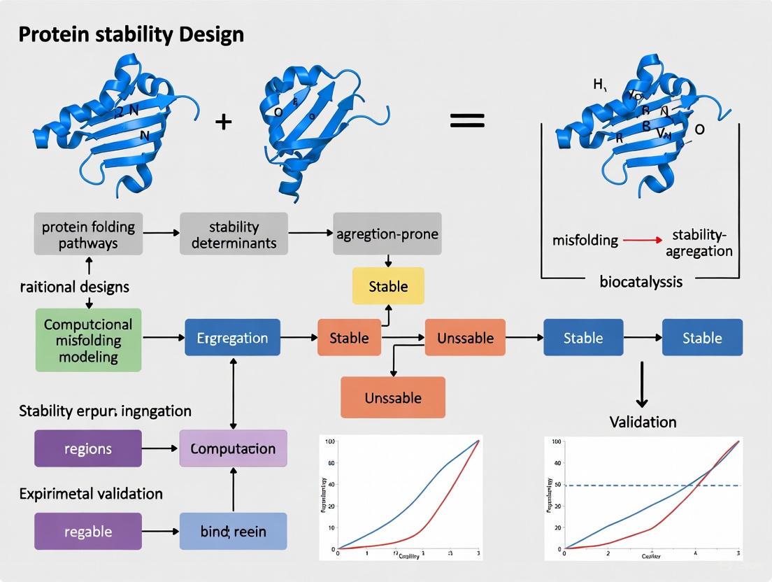
This article provides a comprehensive overview of modern strategies for designing protein stability to prevent misfolding and aggregation, a key pathological mechanism in neurodegenerative diseases and loss-of-function disorders.
Computational Protein Stability Design: Preventing Misfolding and Aggregation for Therapeutics
Abstract
This article provides a comprehensive overview of modern strategies for designing protein stability to prevent misfolding and aggregation, a key pathological mechanism in neurodegenerative diseases and loss-of-function disorders. It explores the foundational principles of protein folding and proteostasis, details cutting-edge computational methodologies from AI-based predictors to physics-based simulations, and addresses critical optimization challenges like the stability-solubility trade-off. Aimed at researchers and drug development professionals, the content synthesizes validation frameworks and comparative analyses of tools to guide the rational design of stable, functional biologics and therapeutics, highlighting the successful translation of these principles into clinical agents.
The Protein Folding Problem: Linking Misfolding to Disease and Cellular Defenses
FAQs: Core Principles and Experimental Challenges
Q1: What is the fundamental thermodynamic principle linking amino acid sequence to protein structure?
The principle, established by Christian Anfinsen's experiments, states that a protein's native three-dimensional structure is the one in which the Gibbs free energy is minimized for a given amino acid sequence and physiological environment [1]. This native conformation is both thermodynamically stable and kinetically accessible. The sequence encodes the folding pathway by defining an energy landscape that resembles a funnel, guiding the polypeptide chain through a multitude of possible conformations toward the lowest-energy state [1]. The same molecular forces that drive proper folding (hydrophobic effect, hydrogen bonding, electrostatics, and van der Waals interactions) can also promote aggregation when partially unfolded states are exposed [2].
Q2: Why is understanding this principle critical for preventing protein aggregation in biopharmaceuticals?
For therapeutic proteins, even minor populations of misfolded or partially unfolded molecules can form stable, irreversible aggregates [2]. These aggregates pose a significant risk as they can elicit deleterious immune responses in patients, potentially leading to drug tolerance or neutralization of the patient's own endogenous proteins [2] [3]. Controlling aggregation is therefore essential for both the efficacy and safety of protein-based drugs. A mechanistic understanding of sequence-dependent aggregation allows for the rational design of more stable therapeutics with reduced immunogenicity [2].
Q3: What are "aggregation hot spots" and how can they be identified?
Aggregation hot spots are short, stretches of amino acids within a protein sequence that are highly prone to forming strong, stable inter-protein contacts [2]. These sequences are typically hydrophobic, lack charges, and have a high propensity to form beta-sheet structures when paired with adjacent strands [2]. They are often buried within the core of the correctly folded native state but become exposed due to local or partial unfolding events. Computational tools can predict these hot spots by analyzing the intrinsic aggregation propensity of the sequence, which aids in the early design stages of therapeutic proteins [2].
Q4: How do experimental conditions impact the thermodynamic stability of a protein?
A protein's folded state is only marginally stable, and its thermodynamic stability is highly sensitive to its environment [2] [3]. Key factors include:
- pH: Changes can alter the charge state of amino acid side chains, disrupting electrostatic and hydrogen-bonding networks.
- Temperature: Increased thermal energy can promote partial unfolding and increase molecular collisions.
- Ionic Strength: Can shield or disrupt electrostatic interactions critical for folding and solubility.
- Interfaces: Exposure to liquid-air or liquid-solid interfaces can induce denaturation.
- Co-solutes: Excipients can either stabilize the native state or destabilize it.
The table below summarizes the mechanisms of instability caused by key environmental factors.
Table 1: Environmental Challenges to Protein Stability and Underlying Mechanisms
| Environmental Factor | Impact on Protein Stability | Molecular Mechanism |
|---|---|---|
| pH Shifts | Charge destabilization, Altered solubility | Modification of ionization states of side chains, disrupting salt bridges and electrostatic interactions [2]. |
| Elevated Temperature | Partial unfolding, Increased aggregation kinetics | Increased kinetic energy overcomes stabilizing weak non-covalent forces, exposing hydrophobic regions [2]. |
| Shear Stress (at interfaces) | Surface-induced denaturation | Unfolding at liquid-air or liquid-solid interfaces, leading to aggregation nucleation [2]. |
| High Protein Concentration | Accelerated aggregation | Increased frequency of molecular collisions, promoting association of partially unfolded species [2]. |
Q5: What are the primary experimental techniques for determining protein structure and stability?
The choice of technique depends on the required resolution, protein size, and the need to study dynamics versus static structure.
Table 2: Key Experimental Techniques for Protein Structure and Stability Analysis
| Technique | Key Application | Throughput | Key Limitations |
|---|---|---|---|
| X-ray Crystallography | High-resolution atomic structure determination | Low | Requires high-quality crystals; possible crystallographic packing artifacts [4]. |
| NMR Spectroscopy | Solution-state structure and dynamics | Medium | Limited by protein size (~25-50 kDa); requires high concentration [4]. |
| Cryo-Electron Microscopy (Cryo-EM) | Large structures and complexes (e.g., viruses, membranes) | Medium-High | Challenging for small proteins (<50 kDa) [4]. |
| Circular Dichroism (CD) | Secondary structure content and stability (thermal/chemical denaturation) | High | Low-resolution; provides structural overview, not atomic details [1]. |
| Differential Scanning Calorimetry (DSC) | Quantitative measurement of thermal stability (Tm and ΔH) | Medium | Requires high protein concentration; can be low-throughput [3]. |
Troubleshooting Guides
Guide 1: Diagnosing and Mitigating Protein Aggregation
Problem: Your therapeutic protein candidate is forming soluble oligomers or visible aggregates during purification or storage.
Investigation & Solution Workflow: The following diagram outlines a systematic approach to diagnose and mitigate aggregation.
Steps:
Analyze Sequence/Structure:
- Action: Use computational tools to identify potential aggregation hot spots and model local stability [2] [5].
- Evidence: Correlate regions of low conformational stability with known proteolytic cleavage sites or hydrogen-deuterium exchange data.
- Solution (Strategy 1 - Engineer Sequence): Implement rational design or directed evolution to introduce stabilizing mutations (e.g., surface entropy reduction, core packing), or disrupt beta-sheet propensity in hot spots without compromising activity [2] [3].
Characterize Solution Conditions:
- Action: Perform a stability screen across a matrix of pH, buffer species, ionic strength, and temperatures. Use techniques like CD, DSC, and size-exclusion chromatography (SEC) to monitor structure and oligomeric state [3].
- Evidence: Identify conditions that maximize the melting temperature (Tm) and minimize the formation of higher molecular weight species.
- Solution (Strategy 2 - Optimize Formulation): Develop the final formulation with optimal pH and include stabilizing excipients such as sugars (e.g., sucrose, trehalose) for preferential exclusion, surfactants (e.g., polysorbate 80) to mitigate interface stress, and antioxidants [3].
Assess Process Stressors:
- Action: Audit the entire production and storage pipeline for stressors like excessive shear (from mixing or pumping), exposure to air-liquid interfaces, freeze-thaw cycles, or metal leachates [2].
- Evidence: Correlate the onset of aggregation with specific unit operations (e.g., after tangential flow filtration).
- Solution (Strategy 3 - Modify Process): Implement process changes such as using lower-shear pumps, adding surfactants early in purification, minimizing bubble formation, and controlling hold times and temperatures [2].
Guide 2: Validating Computational Structure Predictions
Problem: You have used an AI tool like AlphaFold-2 to predict your protein's structure, but need to validate the model experimentally before making drug discovery decisions.
Investigation & Solution Workflow: The following diagram illustrates a multi-technique validation strategy.
Steps:
Low/Medium-Resolution Validation:
- Techniques: Size-exclusion chromatography with multi-angle light scattering (SEC-MALS) to validate oligomeric state; Circular Dichroism (CD) to confirm secondary structure composition; Small-Angle X-ray Scattering (SAXS) to assess overall shape and dimensions [5].
- Interpretation: Does the predicted model have a calculated molecular weight and secondary structure profile that matches experimental data? Does the SAXS-derived envelope fit the predicted model?
High-Resolution Validation (Where Feasible):
- Techniques: X-ray crystallography, Cryo-EM, or NMR spectroscopy [4] [5].
- Interpretation: This provides the most direct and conclusive validation. The atomic coordinates of the experimental structure can be superimposed on the predicted model to calculate root-mean-square deviation (RMSD). An all-atom accuracy of ~1.5 Å RMSD is considered highly accurate [5].
Functional Validation (Essential):
- Techniques: Site-directed mutagenesis of predicted active site or binding interface residues, followed by functional activity assays or binding studies (e.g., Surface Plasmon Resonance - SPR) [5].
- Interpretation: If mutations of computationally predicted critical residues ablates function, this provides strong corroborating evidence for the model's accuracy. This is particularly important for assessing the structure of flexible loops or allosteric sites that may be poorly modeled [5].
The Scientist's Toolkit: Research Reagent Solutions
Table 3: Essential Reagents and Materials for Protein Stability and Aggregation Research
| Reagent/Material | Function | Example Application |
|---|---|---|
| Stabilizing Excipients | Preferentially hydrate the protein surface, shifting equilibrium toward the folded state. | Sucrose, trehalose, sorbitol used in final formulation to enhance shelf-life [3]. |
| Surfactants (e.g., Polysorbate 80) | Compete with protein for interfaces, reducing surface-induced denaturation. | Added to protein solutions to prevent aggregation during pumping, filtration, and shipping [3]. |
| Chaotropes (e.g., Urea, GdnHCl) | Denature proteins by disrupting hydrogen bonding and hydrophobic interactions. | Used in chemical denaturation experiments to measure protein stability (ΔG) and unfolding transitions [1]. |
| Protease Inhibitors | Prevent proteolytic cleavage that can generate truncated, aggregation-prone species. | Added to lysis and purification buffers to maintain protein integrity during isolation [2]. |
| Reducing Agents (e.g., DTT, TCEP) | Maintain cysteine residues in reduced state, preventing incorrect disulfide bond formation. | Critical for handling proteins in non-native environments where disulfide scrambling can occur [3]. |
| Chromatography Resins | Purify protein based on size, charge, or affinity to isolate monodisperse species. | Size-exclusion chromatography (SEC) is essential for separating and quantifying monomeric protein from aggregates [2]. |
| Stability Screening Kits | Enable high-throughput testing of multiple buffer conditions in small volumes. | Used to rapidly identify optimal pH, salt, and excipient conditions for maximizing stability [3]. |
FAQs & Troubleshooting Guide
This section addresses common experimental challenges in proteostasis research, providing targeted solutions based on the molecular mechanisms of the proteostasis network.
FAQ 1: My protein of interest is aggregating during expression and purification. What are the primary cellular systems that should prevent this, and how can I mimic them in vitro?
- Answer: Aggregation occurs when the cellular proteostasis network is overwhelmed or unavailable in vitro. The key is to replicate the function of molecular chaperones, the core components of this network.
- Primary Cellular Defenses:
- Hsp70 System: Binds to hydrophobic patches on nascent or misfolded chains, preventing inappropriate interactions [6] [7]. The ATP-dependent binding and release cycle facilitates proper folding.
- Small Heat Shock Proteins (sHsps): Act as the first line of defense by binding partially folded proteins and preventing them from forming irreversible aggregates, effectively "storing" them for later refolding [8] [9].
- Hsp90 System: Manages the folding and activation of specific "client" proteins, many of which are involved in signaling [7] [9].
- Troubleshooting Steps:
- Reduce Expression Stress: Lower the induction temperature (e.g., to 18-25°C) and use a lower inducer concentration (e.g., 0.1-0.5 mM IPTG) to slow down protein synthesis and give the host cell's chaperones more time to function [7].
- Co-express Chaperones: Co-express your target protein with chaperone systems like Hsp70 (DnaK in E. coli) and its co-chaperones (DnaJ, GrpE) or the GroEL/GroES chaperonin system [7].
- Modify Buffer Conditions In Vitro: Include molecular chaperone mimics in your purification buffers. This can include:
- Non-specific holdases: Add high concentrations of arginine (0.4-0.8 M) or other kosmotropes to suppress protein-protein interactions.
- ATP-regeneration systems: If using purified chaperones like Hsp70, ensure the buffer contains ATP and an ATP-regeneration system (e.g., Creatine Phosphate and Creatine Kinase) to power their folding cycles [6] [9].
- Primary Cellular Defenses:
FAQ 2: How can I experimentally determine if a misfolded protein is being targeted for degradation versus refolding by the proteostasis network?
- Answer: The cell makes a "triage" decision on misfolded proteins, primarily guided by chaperone interactions. You can dissect this pathway using specific inhibitors and tracking methods.
- Experimental Protocol:
- Pulse-Chase Analysis: Metabolically label newly synthesized proteins with a radioactive amino acid (e.g., ^35^S-Methionine) for a short "pulse," then chase with an excess of unlabeled amino acid. Monitor the disappearance of the misfolded protein and the appearance of degradation products over time.
- Inhibitor-Based Pathway Identification:
- For Ubiquitin-Proteasome System (UPS): Treat cells with a proteasome inhibitor like MG-132 or Bortezomib. Accumulation of ubiquitinated forms of your protein (detectable by western blot) indicates it is a UPS substrate [6] [10].
- For Autophagy-Lysosome Pathway (ALP): Treat cells with autophagy inhibitors such as Bafilomycin A1 (inhibits lysosomal acidification) or Chloroquine. Stabilization of your protein suggests ALP-mediated degradation [6] [11].
- Monitor Chaperone Association: Use co-immunoprecipitation to check for stable interactions between your protein and specific chaperones. A persistent interaction with Hsp70, especially in the presence of the co-chaperone CHIP (an E3 ubiquitin ligase), strongly suggests targeting to the UPS for degradation [6] [7].
- Experimental Protocol:
FAQ 3: My research focuses on a neurodegenerative disease model with persistent protein aggregates. What are the known cellular mechanisms for dissolving these aggregates, and why might they be failing?
- Answer: Persistent aggregates indicate a failure in the disaggregation and clearance arms of the proteostasis network.
- Cellular Disaggregation Machinery:
- The Metazoan Disaggregase: Unlike yeast and bacteria which use Hsp104, mammalian cells employ a complex of Hsp70, its nucleotide exchange factor Hsp110, and the J-domain protein Hsp40. This complex can use ATP hydrolysis to forcefully unfold and solubilize protein aggregates [6] [8].
- Post-Disaggregation Triage: After solubilization, proteins are either refolded with chaperone assistance or, if refolding fails, ubiquitinated and degraded [8].
- Reasons for Failure:
- Overwhelming Aggregate Load: In diseases like Alzheimer's and Parkinson's, the sheer volume of aggregates (e.g., Aβ, α-synuclein) may exceed the capacity of the disaggregation machinery [11] [12].
- Age-Related Decline: The expression and activity of key proteostasis network components, including Hsp70, decline with age, which is the primary risk factor for most neurodegenerative diseases [11] [7].
- Sequestration of Machinery: The aggregates themselves can actively sequester essential chaperones and proteasome components, functionally depleting the cell's ability to respond to proteotoxic stress [11] [7].
- Experimental Approach: Quantify the mRNA and protein levels of key disaggregation components (Hsp70, Hsp110, Hsp40) in your disease model versus controls. A knockdown or knockout of these components in your model should exacerbate the aggregation phenotype, confirming their functional role.
- Cellular Disaggregation Machinery:
FAQ 4: What are the key differences in how the proteostasis network handles cytosolic protein misfolding versus misfolding in the endoplasmic reticulum (ER)?
- Answer: While the core principles are similar, the compartments use distinct machineries and signaling pathways.
- Cytosolic Misfolding:
- Endoplasmic Reticulum Misfolding (ERAD):
- Primary Chaperones: BiP (an Hsp70 homolog), Calnexin/Calreticulin (for glycoproteins) [1] [11].
- Degradation Pathway: ER-associated degradation (ERAD). Misfolded proteins are retro-translocated into the cytosol, ubiquitinated, and degraded by the proteasome [1] [11].
- Stress Response: The Unfolded Protein Response (UPR), which has three main sensors (IRE1, PERK, ATF6) that work to reduce protein load and increase folding capacity in the ER [1] [11].
The table below summarizes the quantitative data on proteostasis network associations with major disease classes, highlighting key therapeutic targets.
Table 1: Proteostasis Network Signatures in Human Diseases. Data derived from large-scale pan-disease analysis showing the over-representation of proteostasis network components in disease gene sets [10].
| Disease Category | Fraction of Disease Gene Set Composed of Proteostasis Proteins | Key Over-Represented Pathways | Key Over-Represented Functional Classes |
|---|---|---|---|
| Cancer | 25% - 36% | UPS, Autophagy-Lysosome Pathway (ALP) | UPS E3 Ligases, Transcription Factors |
| Neurodegenerative Diseases | 30% - 35% | UPS, ALP, Extracellular Proteostasis | Molecular Chaperones, UPS Ubiquitin-Binding Proteins |
| Cardiovascular, Autoimmune, Endocrine | 20% - 30% | ALP, Extracellular Proteostasis | Molecular Chaperones, Transcription Factors |
Key Experimental Protocols
This section provides detailed methodologies for critical experiments investigating chaperone function and protein quality control.
Protocol 1: Assessing Protein Disaggregation Activity In Vitro
- Objective: To reconstitute and measure the disaggregation of a model protein aggregate by the Hsp70/Hsp110/Hsp40 chaperone system.
- Background: This protocol tests the function of the core metazoan disaggregation machinery, which is crucial for reversing protein aggregation in neurodegenerative disease models [6] [8].
- Materials:
- Purified chaperones: Hsp70, Hsp110 (NEF), Hsp40 (J-protein).
- Model substrate (e.g., heat-denatured, aggregated Luciferase or GFP).
- ATP-regeneration system (ATP, Creatine Phosphate, Creatine Kinase).
- Reaction buffer (e.g., 40 mM HEPES-KOH pH 7.4, 50 mM KCl, 5 mM MgCl2).
- Thermoshaker and plate reader (for luciferase/GFP activity).
- Methodology:
- Prepare Aggregated Substrate: Denature the model protein (e.g., 2 µM Luciferase) by heating at 42°C for 20-30 minutes. Confirm aggregation by dynamic light scattering or turbidity measurement.
- Set Up Disaggregation Reaction: In a reaction tube, combine:
- Reaction buffer.
- ATP-regeneration system (1-2 mM ATP, 10 mM Creatine Phosphate, 0.1 µM Creatine Kinase).
- Aggregated substrate.
- Chaperone mix (e.g., 2-5 µM Hsp70, 1-2 µM Hsp110, 1-2 µM Hsp40).
- Incubate and Monitor: Incubate the reaction at 30-37°C. For luciferase, take aliquots at regular intervals (e.g., 0, 15, 30, 60, 90, 120 min) and measure recovered enzymatic activity using a luminometer upon adding substrate. For GFP, monitor fluorescence recovery over time.
- Controls: Include essential negative controls: a reaction with no ATP and a reaction missing one key chaperone (e.g., Hsp110).
- Data Analysis: Plot the percentage of recovered activity over time. A successful disaggregation reaction will show a time-dependent increase in signal, dependent on the presence of all chaperones and ATP.
Protocol 2: Differentiating Degradation Pathways for a Misfolded Protein
- Objective: To determine whether a misfolded protein of interest is degraded by the proteasome or via autophagy in living cells.
- Background: Misfolded proteins are triaged for degradation primarily by the UPS or ALP. Identifying the correct pathway is essential for understanding disease mechanisms and designing interventions [6] [10].
- Materials:
- Cell line expressing your protein of interest.
- Cycloheximide (protein synthesis inhibitor).
- Proteasome inhibitor (e.g., MG-132, 10-20 µM).
- Autophagy/Lysosome inhibitor (e.g., Bafilomycin A1, 100 nM).
- Antibodies for your protein and a loading control (e.g., GAPDH, Tubulin).
- Methodology:
- Treat Cells: Split cells into four treatment groups in 6-well plates:
- Group 1 (Control): DMSO vehicle control.
- Group 2 (Proteasome Inhibition): MG-132.
- Group 3 (Autophagy Inhibition): Bafilomycin A1.
- Group 4 (Dual Inhibition): MG-132 + Bafilomycin A1.
- Block New Synthesis: After pre-treating with inhibitors for 1 hour, add Cycloheximide (50-100 µg/mL) to all groups to stop new protein synthesis. This allows you to monitor the decay of the existing protein pool.
- Harvest and Analyze: Harvest cells at specific time points after Cycloheximide addition (e.g., 0, 2, 4, 8 hours). Prepare whole-cell lysates and perform a western blot for your protein of interest.
- Quantify: Quantify the band intensity relative to the loading control and the time-zero point.
- Treat Cells: Split cells into four treatment groups in 6-well plates:
- Data Interpretation:
- If the protein stabilizes (decays slower) only with MG-132, it is primarily a UPS substrate.
- If it stabilizes only with Bafilomycin A1, it is primarily an autophagy substrate.
- If it stabilizes most significantly with dual inhibition, it is likely degraded by both pathways.
Proteostasis Network Signaling Pathways
The following diagrams illustrate the key signaling pathways that regulate the proteostasis network, central to experimental design in protein stability research.
Cytosolic Heat Shock Response
Chaperone-Mediated Protein Triage
The Scientist's Toolkit: Research Reagent Solutions
This table details essential reagents for studying molecular chaperones and protein quality control, with explanations of their specific functions in experimental contexts.
Table 2: Essential Research Reagents for Proteostasis Network Studies
| Research Reagent | Function / Mechanism of Action | Key Experimental Use |
|---|---|---|
| MG-132 / Bortezomib | Reversible inhibitors that bind the proteasome's catalytic subunits, blocking chymotryptic activity. | To determine if a protein is degraded by the UPS. Stabilization of the protein upon treatment indicates it is a proteasome substrate [6] [10]. |
| Bafilomycin A1 | A specific vacuolar-type H+-ATPase (V-ATPase) inhibitor. Prevents lysosomal acidification, blocking autophagic degradation. | To inhibit the Autophagy-Lysosome Pathway (ALP). Used to distinguish ALP-dependent degradation from UPS-dependent degradation [6] [11]. |
| Recombinant Chaperone Proteins (Hsp70, Hsp40, Hsp110) | Purified, active human or bacterial chaperones. Function in an ATP-dependent manner to bind, refold, or disaggregate substrate proteins in vitro. | For in vitro reconstitution assays to study the mechanism of protein folding, disaggregation, and the specific roles of individual chaperones in these processes [6] [8] [9]. |
| ATP-Regeneration System | A cocktail of ATP, creatine phosphate, and creatine kinase. The kinase continuously regenerates ATP from ADP using the phosphate donor, maintaining constant ATP levels. | Essential for any in vitro chaperone assay (folding, disaggregation) as most chaperones are ATP-dependent enzymes. Prevents artifact from ATP depletion [9]. |
| HSF1 Activators (e.g., Celastrol) | Small molecules that activate the Heat Shock Transcription Factor 1 (HSF1), leading to upregulated expression of endogenous chaperones like Hsp70. | To test whether boosting the cell's intrinsic proteostasis capacity can alleviate protein misfolding and aggregation in cellular disease models [7]. |
| Clusterin | An extracellular holdase chaperone that binds to a wide range of misfolded proteins, including Aβ and α-synuclein, to prevent their aggregation. | Used in vitro and in cell models to study the suppression of amyloid formation and to investigate the role of extracellular proteostasis in protein aggregation diseases [9]. |
Protein homeostasis, or proteostasis, is fundamental to cellular health. It represents the delicate balance between protein synthesis, folding, trafficking, and degradation that maintains a functional proteome [13]. When this balance is disrupted—through genetic mutations, cellular stress, or aging—proteins may misfold and aggregate, leading to a pathological state known as dysproteostasis [13]. In neurodegenerative diseases and loss-of-function disorders, this aggregation process is not merely a secondary symptom but a primary driver of pathology, contributing to both toxic gain-of-function effects and critical loss of normal cellular activities [14] [15] [16]. This technical support center provides troubleshooting guidance and foundational knowledge for researchers investigating these complex mechanisms, framed within the broader context of designing stable proteins to prevent misfolding and aggregation.
Frequently Asked Questions (FAQs): Core Concepts
1. What is the fundamental link between protein misfolding and aggregation in neurodegenerative diseases?
Proteins fold into specific three-dimensional structures to perform their biological functions. The "thermodynamic hypothesis," established by Christian Anfinsen's work, states that a protein's native structure is determined by its amino acid sequence and represents the most thermodynamically stable conformation under physiological conditions [13]. Misfolding occurs when polypeptides deviate from this correct folding pathway, often due to factors like genetic mutations or oxidative stress [13] [17]. These misfolded proteins can then self-assemble into aggregates. In major neurodegenerative conditions like Alzheimer's disease, Parkinson's disease, and amyotrophic lateral sclerosis (ALS), specific proteins such as amyloid-β, tau, α-synuclein, and TAR DNA-binding protein 43 (TDP-43) form amyloid fibrils that undergo prion-like propagation throughout the nervous system, ultimately inducing neurodegeneration [14].
2. How can protein aggregation simultaneously cause gain-of-function and loss-of-function pathologies?
Aggregation can lead to a dual pathology: a toxic gain-of-function from the aggregated protein itself and a critical loss-of-function due to the depletion of the normal, functional protein.
- Gain-of-Function: The aggregates themselves can be toxic. They may disrupt cellular membranes, impair the function of organelles, and overwhelm the cellular protein quality control systems [17]. For instance, cytoplasmic TDP-43 inclusions recruit essential proteins, sequestering them away from their normal functions [16] [18].
- Loss-of-Function: The aggregation process depletes the pool of functional, soluble protein. In the nucleus, depletion of TDP-43 leads to a loss of its normal role in RNA metabolism, resulting in aberrant cryptic splicing and disrupted gene expression, which is a direct loss-of-function pathology [16] [18]. Similarly, a 2025 study on GGC repeat disorders showed that polyglycine aggregates specifically recruit and deplete the tRNA ligase complex, disrupting essential tRNA processing and mimicking genetic tRNA splicing disorders [19].
3. What are the primary molecular mechanisms by which genetic mutations cause disease through protein aggregation?
Disease-causing mutations in protein-coding regions can be broadly categorized into three molecular mechanisms, each with distinct therapeutic implications [15]:
- Loss-of-Function (LOF): Mutations (e.g., premature stop codons or destabilizing missense changes) lead to a reduction or complete absence of the protein's normal activity. Therapeutic strategies often aim to replace or compensate for the missing function, such as with gene therapy [15].
- Gain-of-Function (GOF): Mutations cause the protein to acquire a new, often toxic, function or increased activity. This includes forming toxic aggregates. Therapies typically involve inhibiting the mutant protein's function using small molecules or gene silencing [15].
- Dominant-Negative (DN): The mutant protein interferes with the function of the wild-type protein, for example, by forming dysfunctional complexes. Therapeutic approaches may involve allele-specific targeting to silence the mutant allele [15]. A 2025 study estimated that dominant-negative and gain-of-function mechanisms account for 48% of phenotypes in dominant genes, highlighting the prevalence of non-LOF mechanisms in aggregation diseases [15].
4. Beyond neurodegeneration, what are some unexpected cellular functions affected by protein aggregation?
Recent research has revealed novel and unexpected pathways disrupted by aggregation. The 2025 study on GGC repeat disorders demonstrated that polyglycine aggregates do not just cause generic cellular stress but can specifically sequester the tRNA ligase complex (tRNA-LC) [19]. This recruitment depletes the cell of functional tRNA-LC, leading to misprocessed tRNAs and disrupting global protein synthesis. This mechanism directly links protein aggregation to RNA processing disorders and explains the selective neuronal vulnerability observed in these diseases [19].
Troubleshooting Guides
Guide 1: Addressing Common Protein Solubility and Aggregation Issues in Vitro
Problem: Your recombinant protein is forming aggregates or precipitating during expression, purification, or storage.
Solution: A systematic approach to optimize buffer conditions and protein handling.
| Issue Area | Possible Cause | Recommended Action | Theoretical Basis |
|---|---|---|---|
| Buffer Conditions | Non-optimal pH or ionic strength leading to instability. | Adjust pH to the protein's stable point (often near its isoelectric point). Modulate ionic strength; add salts like NaCl to shield electrostatic attractions. | Solubility is highly dependent on the protein's net charge and the electrostatic environment [20]. |
| Physical Stress | Exposure to high temperatures, shaking, or air-liquid interfaces. | Work at lower temperatures (4°C). Avoid vigorous shaking; use gentle pipetting. Add non-denaturing detergents for membrane proteins. | Proteins can become unstable and denature at high temperatures or due to surface-induced stresses, initiating the aggregation pathway [21]. |
| Additives | Lack of stabilizing agents in the solution. | Include additives like glycerol, polyethylene glycol (PEG), or amino acids (e.g., arginine). Test different molecular chaperones. | These additives can stabilize proteins by providing a more favorable chemical environment, reducing protein-protein interactions, or actively assisting folding [20]. |
| Protein Sequence | Hydrophobic residues on the protein surface promoting interaction. | Use site-directed mutagenesis to replace surface hydrophobic residues with hydrophilic ones. | This reduces the hydrophobic interactions that are a primary driver of protein aggregation [20]. |
| Expression System | Incorrect folding in a non-optimal host (e.g., E. coli). | Switch expression system (e.g., yeast, insect, or mammalian cells) to obtain necessary post-translational modifications and chaperones. | Different host systems offer varying components of the proteostasis network, which is crucial for proper folding [20]. |
Experimental Protocol: Refolding Proteins from Inclusion Bodies If solubility cannot be achieved and the protein is trapped in inclusion bodies, refolding is a potential solution [20].
- Solubilization: Isolate inclusion bodies and solubilize the aggregated protein using a strong denaturant, such as 6-8 M guanidine hydrochloride or 8 M urea.
- Purification: Purify the denatured protein under denaturing conditions if possible (e.g., using affinity chromatography).
- Refolding: Dilute the denatured protein slowly into a refolding buffer. This buffer should contain:
- A redox system (e.g., reduced/oxidized glutathione) to facilitate disulfide bond formation.
- Stabilizing additives like arginine, glycerol, or PEG.
- A pH and salt concentration optimized for the target protein.
- Concentration and Characterization: Concentrate the refolded protein and thoroughly characterize its activity and monodispersity using techniques like size-exclusion chromatography and circular dichroism.
Guide 2: Selecting Analytical Techniques for Protein Aggregate Characterization
Problem: You need to characterize the size, amount, and type of aggregates in your protein sample, but the available techniques are numerous and varied.
Solution: Employ a combination of orthogonal methods to cover the wide size range and different properties of protein aggregates. The table below summarizes key techniques. No single method can provide a complete picture; a strategic combination is essential [21].
| Method | Principle | Size Range | Key Information | Main Consideration |
|---|---|---|---|---|
| Dynamic Light Scattering (DLS) | Fluctuations in scattered light due to Brownian motion. | 1 nm - 6 μm | Hydrodynamic size distribution, sample homogeneity. | Does not resolve complex mixtures well; sensitive to dust/large particles. |
| Analytical Ultracentrifugation (AUC) | Sedimentation under high centrifugal force. | ~0.1 nm - 1 μm | Mass and shape information; can separate and quantify species. | Low throughput; requires significant expertise and data analysis. |
| Size-Exclusion Chromatography (SEC) | Size-based separation of molecules in solution. | ~1 - 30 nm (hydrodynamic radius) | Quantification of soluble aggregates (dimers, trimers) relative to monomer. | May not detect large aggregates that stick to the column matrix. |
| Micro-Flow Imaging / Flow Microscopy | Microscopic imaging of particles in a flow cell. | 1 - 400 μm | Concentration, size, and morphology of particles; can differentiate protein from other particles. | Generates large data volumes; emerging technique for subvisible particles. |
| Native Gel Electrophoresis | Separation by size and charge under non-denaturing conditions. | Varies | Identification of soluble oligomeric species. | Semi-quantitative; may not be suitable for very large aggregates. |
The following workflow diagram illustrates a recommended strategy for characterizing protein aggregates throughout product development, from early discovery to quality control, based on guidance from the European Immunogenicity Platform [21].
The Scientist's Toolkit: Research Reagent Solutions
| Reagent / Material | Function / Application | Key Consideration |
|---|---|---|
| Molecular Chaperones (e.g., Hsp70, Hsp40, Hsp104) | Assist in proper protein folding, prevent aggregation, refold misfolded proteins, and disaggregate existing aggregates [13] [17]. | Hsp104 is present in yeast and crucial for prion propagation but absent in metazoans, where disaggregation is handled by Hsp70/Hsp40/Hsp110 systems [17]. |
| TDP-43 Low-Complexity Domain Fibrils | Pre-formed amyloid-like fibrils used to seed TDP-43 aggregation in cellular models (e.g., iPSC-derived neurons) to study ALS/FTD pathology [16] [18]. | This model robustly recapitulates both cytoplasmic inclusion formation and nuclear loss-of-function, key hallmarks of TDP-43 proteinopathies. |
| Small Molecule Chaperone Modulators | Pharmacologically manipulate the proteostasis network. For example, small molecule Hsp90 inhibitors have shown success in ameliorating tau and Aβ burden in models of Alzheimer's disease [17]. | The pharmacology of current scaffolds can be challenging, driving research into targeting specific co-chaperones for improved specificity [17]. |
| Site-Directed Mutagenesis Kits | Systematically replace hydrophobic surface residues with hydrophilic ones to engineer proteins with enhanced solubility and reduced aggregation propensity [20]. | Requires prior structural knowledge to avoid disrupting the protein's active site or core functional domains. |
| tRNA Ligase Complex (tRNA-LC) Components | Key reagents for studying a novel aggregation pathway in GGC repeat disorders, where polyglycine aggregates sequester tRNA-LC, disrupting tRNA processing and leading to neurodegeneration [19]. | Studying this complex provides a direct link between protein aggregation and RNA processing defects, revealing a new therapeutic target. |
FAQs: Troubleshooting Common Experimental Challenges
Q1: My HSP90 inhibition experiment is producing unexpected results in a Hepatovirus model. Could previous assumptions about its necessity be incorrect?
A1: Yes, recent research has overturned the long-held assumption that Hepatitis A virus (HAV) replication is independent of HSP90. If your experiments are not showing an effect, consider the inhibitor concentration and model system.
- Key Evidence: A 2025 study demonstrates that HAV replication is highly dependent on HSP90 chaperone activity, both in human hepatocyte-derived cell lines and in vivo mouse models. The 50% inhibitory concentration (IC50) of the HSP90 inhibitor geldanamycin was found to be very low (8.7-11.8 nM), indicating high potency [22].
- Troubleshooting Tip: Ensure you are using a potent and specific HSP90 inhibitor at an appropriate concentration. The previous hypothesis that HAV's slow translational kinetics made it HSP90-independent has been refuted; it is now considered more dependent on HSP90 than some other picornaviruses [22].
Q2: I am engineering cell factories for therapeutic protein production, but sustained UPR activation is leading to high apoptosis. How can I dynamically control this response to improve yields?
A2: Static overexpression of UPR components often fails due to cellular adaptation and toxicity. Implement a feedback-responsive system that senses proteotoxic stress and modulates the UPR dynamically.
- Recommended Protocol: Engineer sense-and-respond circuits that:
- Expected Outcome: This dynamic control, as demonstrated with tissue plasminogen activator (tPA) and blinatumomab, enhances cell viability and increases the production of functional, secreted protein by aligning UPR modulation with real-time folding demands [23].
Q3: Can modulating the Unfolded Protein Response (UPR) be a viable strategy for treating complex neurodegenerative diseases like ALS/FTD?
A3: Emerging evidence suggests that artificially enforcing a specific arm of the UPR could be a promising pan-therapeutic strategy for diseases characterized by proteostasis failure.
- Experimental Insight: Intracerebroventricular administration of AAVs to express the active, spliced form of XBP1 (XBP1s) in ALS/FTD models improved motor performance, extended lifespan, and reduced protein aggregation. This was effective in models of SOD1, TDP-43, and C9orf72 pathogenesis [24].
- Mechanism: XBP1s is a master transcription factor that upregulates genes involved in ER protein folding, quality control, and degradation. Its overexpression compensates for the suboptimal UPR activation observed in these disease models, improving overall proteostasis [24].
Q4: How can I accurately measure the effects of thousands of mutations on protein folding stability in a high-throughput manner?
A4: Traditional methods are low-throughput. Implement the cDNA display proteolysis method, which can measure thermodynamic folding stability for up to hundreds of thousands of protein variants in a single experiment [25].
- Workflow Summary:
- Create a DNA library of your protein variants.
- Use cell-free cDNA display to create protein-cDNA complexes.
- Incubate with a series of protease concentrations. Folded proteins are protease-resistant.
- Pull down intact proteins and use deep sequencing to quantify survival rates for each sequence.
- Apply a kinetic model to infer thermodynamic folding stability (ΔG) from the sequencing data [25].
- Advantage: This method is fast, accurate, and uniquely scalable, allowing you to uncover the quantitative rules of how sequence encodes stability [25].
Table 1: HSP90 Inhibitors in Antiviral and Neurological Research
| Inhibitor Name | Target | Key Experimental Context | Potency (IC50/Kd) | Key Findings & Applications |
|---|---|---|---|---|
| Geldanamycin [22] | HSP90 | Hepatitis A Virus (HAV) Replication | 8.7-11.8 nM | Potently blocks HAV replication in vitro and in vivo; more potent for HAV than other picornaviruses [22]. |
| [11C]HSP990 [26] | HSP90 (Brain) | PET Neuroimaging in Neurodegeneration | Kd = 1.6 nM (Human brain homogenate) | Successful PET tracer for quantifying brain Hsp90; shows reduced binding in Alzheimer's model brain tissue [26]. |
| [11C]BIIB021 [26] | HSP90 (Brain) | PET Neuroimaging | Information in source | Exhibits Hsp90-specific binding in rat brain; presence of brain radiometabolites complicates quantification [26]. |
| PU-AD [26] | HSP90 | Therapeutic / Imaging for Alzheimer's | Information in source | Showed promise in preclinical studies; evaluated in clinical trials (withdrawn/terminated) [26]. |
Table 2: High-Throughput Protein Folding Stability Analysis (cDNA Display Proteolysis)
| Parameter | Specification | Relevance for Experimental Design |
|---|---|---|
| Throughput [25] | ~900,000 protein domains per one-week experiment | Enables comprehensive mutational scans and stability landscapes. |
| Cost [25] | ~$2,000 per library (excluding DNA synthesis/sequencing) | Cost-effective for the scale of data generated. |
| Data Accuracy [25] | R = 0.94 (between trypsin & chymotrypsin experiments) | High reproducibility and reliability of inferred ΔG values. |
| Typical Library [25] | All single amino acid variants and selected double mutants of 331 natural and 148 de novo designed domains | Provides a uniform, comprehensive dataset for machine learning and biophysical analysis. |
Key Experimental Protocols
Protocol 1: Assessing HSP90 Dependency in Viral Replication Using Inhibitors
This protocol is adapted from research confirming HSP90's critical role in Hepatitis A virus replication [22].
- Cell Culture and Infection: Use relevant host cells (e.g., human hepatocyte-derived cell lines). Infect with the virus of interest at an appropriate multiplicity of infection (MOI).
- Inhibitor Treatment: Prepare a dilution series of a validated HSP90 inhibitor (e.g., geldanamycin). Treat cells with the inhibitor concurrently with or shortly after viral infection. Include a DMSO vehicle control.
- Cytotoxicity Assay: Perform a parallel cytotoxicity assay (e.g., MTT, LDH) to ensure that antiviral effects are not due to general cell death. The IC50 for viral inhibition should be significantly lower than the cytotoxic concentration.
- Replication Quantification:
- For productive infection: Measure viral titers using plaque assays or TCID50 at 24-48 hours post-infection.
- For replication mechanisms: Use subgenomic replicon systems to directly assess the role of HSP90 in RNA amplification independent of capsid assembly [22].
- Downstream Analysis: To probe the mechanism, perform label-free quantitative proteomics to identify which viral proteins (e.g., capsid precursors) interact with HSP90 [22].
Protocol 2: Engineering Feedback-Responsive Cell Factories for Dynamic UPR Control
This protocol outlines the creation of engineered cells that autonomously manage ER stress to enhance recombinant protein production [23].
- Sensor Construction: Create an ER stress sensor by placing a transcriptional regulator (e.g., tTA) under the control of a UPR target promoter, such as the one for the XBP1s-target gene ERdj4 [23].
- Actuator Engineering:
- For Stress Attenuation: Design a circuit where the sensor activates expression of the active transcription factor XBP1s, creating a positive feedback loop to amplify the pro-folding arm of the UPR [23].
- For Apoptosis Delay: Design a separate circuit where the sensor drives expression of a repressor that targets the pro-apoptotic gene CHOP [23].
- Cell Line Generation: Stably integrate these sense-and-respond circuits into your production cell line (e.g., CHO or HEK293).
- Validation and Production:
- Characterization: Induce recombinant protein expression and use fluorescent reporters to monitor the dynamic activation of the sensor and actuator pathways over time.
- Performance Metrics: Compare cell viability, duration of protein production, and final functional titer of the therapeutic protein (e.g., tPA or bispecific antibodies) against control cell lines lacking the dynamic circuits [23].
Signaling Pathway Diagrams
Diagram 1: Integrated Cellular Stress Response Pathways
Diagram 2: cDNA Display Proteolysis Workflow
The Scientist's Toolkit: Research Reagent Solutions
Table 3: Essential Reagents for Stress Response Research
| Reagent / Tool | Function / Application | Key Characteristics |
|---|---|---|
| HSP90 Inhibitors (e.g., Geldanamycin, 17-AAG) [22] [27] | Probing HSP90 function in viral replication, cancer, and neurodegeneration. | Potent, ATP-competitive inhibitors. Used to dissect chaperone-client relationships and as therapeutic leads. |
| UPR Reporter Cell Lines [23] | Quantifying activation of specific UPR branches (IRE1, PERK) in real-time. | Typically use GFP under control of UPR target promoters (e.g., ERdj4 for IRE1, CHOP for PERK). Enable dynamic, single-cell resolution. |
| cDNA Display Proteolysis Kit (Conceptual) [25] | High-throughput measurement of protein folding stability for vast variant libraries. | Components for cell-free translation, protease digestion, and cDNA-protein pull-down. Requires NGS capabilities. |
| AAV-XBP1s Vectors [24] | Gene therapy approach to artificially enforce the adaptive UPR in disease models. | Used to deliver the active XBP1s transcription factor to tissues (e.g., CNS) to improve proteostasis and reduce aggregation. |
| Hsp90 PET Tracers (e.g., [11C]HSP990) [27] [26] | Non-invasive in vivo visualization and quantification of Hsp90 expression in the brain. | Critical for validating target engagement of Hsp90 drugs in the CNS and as potential diagnostic biomarkers for neurodegeneration. |
Computational Arsenal: AI, Physics, and De Novo Design for Stable Proteins
Welcome to the Technical Support Center
This support center is designed for researchers and scientists employing machine learning predictors for protein stability design. The guides and FAQs below will help you troubleshoot specific issues encountered while using RaSP or meta-predictors in experiments aimed at preventing pathogenic protein misfolding and aggregation.
Frequently Asked Questions (FAQs)
General Predictor Concepts
Q1: What is the core difference between a meta-predictor and a tool like RaSP?
A meta-predictor integrates the predictions of multiple independent computational tools to form a single, consensus prediction. This approach mitigates the individual biases and limitations of any single tool. For instance, one study combined 11 different tools into a meta-predictor, which demonstrated improved performance and reliability over any individual component [28].
In contrast, RaSP (Rapid Stability Prediction) is a specific, deep learning-based method. It uses a self-supervised 3D convolutional neural network to learn representations of protein structure, which is then fine-tuned in a supervised manner to predict changes in thermodynamic stability (ΔΔG) on an absolute scale [29].
Q2: Why might my predicted stabilizing mutation still cause the protein to aggregate?
This is a common challenge. Computational tools often increase predicted stability by recommending mutations that increase the hydrophobicity of the protein surface. While this can improve stability, it frequently does so at the cost of solubility, leading to aggregation. Analysis of a large mutation dataset confirmed that stabilizing mutations on the protein surface are strongly correlated with increased hydrophobicity [28]. Always check if a predicted stabilizing mutation introduces hydrophobic residues in solvent-exposed areas.
RaSP-Specific Workflow
Q3: What is the typical workflow for running a RaSP analysis, and where do errors most often occur?
The standard workflow and common failure points are outlined below. Errors most frequently occur during the input preparation stage, specifically with incorrect PDB file formatting or selection.
Q4: RaSP is reporting high errors for specific amino acid substitutions. Is this a known issue?
Yes, the accuracy of RaSP is not uniform across all mutation types. The model exhibits larger prediction errors when substituting glycine residues or when changing residues to proline. This is likely due to the unique conformational constraints these amino acids impose [29]. Treat predictions involving these residues with extra caution.
Meta-Predictor Specifics
Q5: Which individual tools are commonly integrated into a stability meta-predictor?
A proven meta-predictor can incorporate a diverse set of tools. The following table lists tools that have been successfully combined, leveraging their complementary strengths for different mutation types [28].
| Tool Name | Underlying Methodology | Key Strengths / Profile |
|---|---|---|
| FoldX | Empirical Force Field | Accurate for mutations increasing hydrophobicity [28] |
| Rosetta-ddG | Empirical & Physical Force Field | Accurate for mutations increasing hydrophobicity [28] |
| EGAD | Physical Force Field | Accurate for mutations increasing hydrophobicity [28] |
| PoPMuSiC | Statistical Potential | Accurate for mutations that reduce or do not change hydrophobicity [28] |
| CUPSAT | Statistical Potential | Accurate for mutations that reduce or do not change hydrophobicity [28] |
| SDM | Statistical Potential | Accurate for mutations that reduce or do not change hydrophobicity [28] |
| DFire | Statistical Potential | Good overall performance, especially on buried residues [28] |
| IMutant3 | Machine Learning/Neural Network | Less reliable for surface-exposed residues [28] |
Troubleshooting Guides
Issue 1: Predictions Contradict Experimental Stability Data
Problem: Your in silico screening identifies mutations predicted to be highly stabilizing, but subsequent experimental characterization (e.g., thermal shift assays) shows they are neutral or even destabilizing.
Solution:
- Verify Structural Context: The accuracy of most predictors, including RaSP and tools within a meta-predictor, is highest for buried residues and lower for surface-exposed ones [28]. Check the location of your mutated residue.
- Check for Functional/Allosteric Residues: A mutation might be structurally stabilizing but disrupt allosteric networks or functional sites. Avoid residues implicated in function, such as active sites or binding pockets. In one case, excluding 21 functional residues was crucial for maintaining the glycan-binding capacity of ThreeFoil while stabilizing it [28].
- Audit Your Input Structure: Ensure the protein structure file (PDB) used for prediction is of high resolution and relevant to your experimental conditions. Mismatches here are a common source of discrepancy.
- Consider the Solubility Trade-off: The mutation may indeed increase thermodynamic stability but cause aggregation, which can be misinterpreted as instability in some assays. Run complementary aggregation predictors or inspect the mutation for increased surface hydrophobicity [28].
Issue 2: Handling the Stability-Solubility Trade-off
Problem: Successfully designed stabilized protein variants show a tendency to aggregate, reducing yield and usability for therapeutic or biotechnological applications.
Solution:
- Post-Prediction Filtering: After generating a list of candidate stabilizing mutations, filter out those that:
- Increase hydrophobicity on the protein surface.
- Reduce net charge or create patches of neutral charge.
- Prioritize Core Mutations: Focus stabilization efforts on residues that are buried in the protein core, as these are less likely to negatively impact solubility [28].
- Iterative Design: Use the stabilized variant as a new backbone and run further prediction rounds, explicitly filtering for solubility. Machine learning models are increasingly being trained to recognize this balance.
Issue 3: RaSP Model Performance and Validation
Problem: You need to understand the expected performance and limitations of the RaSP model to justify its use in your study or a publication.
Solution: Refer to the published benchmarks of RaSP against experimental and computational data. The table below summarizes key performance metrics [29].
| Validation Data Set | RaSP vs. Rosetta Correlation (Pearson ρ) | RaSP vs. Experimental Data Correlation (Pearson ρ) |
|---|---|---|
| RaSP Test Set (10 proteins) | 0.71 - 0.88 | - |
| Myoglobin (1BVC) | 0.91 | 0.71 |
| Lysozyme (1LZ1) | 0.80 | 0.57 |
| Protein G (1PGA) | 0.90 | 0.72 |
| NUDT15 (5BON) | 0.83 | 0.50 |
| PTEN (1D5R) | 0.87 | 0.52 |
The Scientist's Toolkit: Research Reagent Solutions
| Essential Material / Resource | Function in Experiment | Technical Notes |
|---|---|---|
| Target Protein Structure (PDB file) | Serves as the input for all structure-based prediction tools (RaSP, FoldX, Rosetta). | Use high-resolution (<2.5 Å) crystal structures. Consider the biological relevance of the specific conformation. |
| RaSP Web Server / Code | Provides rapid (sub-second per residue) predictions of ΔΔG for saturation mutagenesis. | Freely available via a web interface or local installation for large-scale analyses [29]. |
| Meta-Predictor Web Server | Combines multiple tools (e.g., FoldX, Rosetta, PoPMuSiC) to generate a consensus stability prediction. | An example implementation is available at meieringlab.uwaterloo.ca/stabilitypredict/ [28]. |
| Thermal Denaturation Assay | Experimentally validates the change in melting temperature (ΔTm) of designed variants. | The gold-standard for measuring changes in thermodynamic stability. Correlate ΔTm with predicted ΔΔG. |
| Size-Exclusion Chromatography (SEC) | Assesses the solubility and aggregation state of stabilized protein variants. | Critical for identifying the stability-solubility trade-off. A stable but aggregated protein will show an altered elution profile. |
Experimental Protocol: Validating Predictor Output
This protocol describes a standard method for experimentally testing computationally predicted stabilizing mutations.
1. Protein Expression and Purification:
- Clone the gene for your wild-type and mutant proteins into an appropriate expression vector.
- Express the proteins in your chosen system (e.g., E. coli).
- Purify the proteins using affinity and size-exclusion chromatography to ensure homogeneity.
2. Thermodynamic Stability Assay (Differential Scanning Fluorimetry - DSF):
- Principle: This high-throughput method measures protein unfolding by monitoring a fluorescent dye that binds to hydrophobic patches exposed upon denaturation.
- Procedure:
- Mix purified protein with a fluorescent dye (e.g., SYPRO Orange) in a quantitative PCR plate.
- Gradually increase the temperature (e.g., from 25°C to 95°C) while measuring fluorescence.
- Generate a melt curve for each variant. The midpoint of this curve is the melting temperature (Tm).
- Analysis: A higher Tm for a mutant compared to the wild-type indicates increased stability. The change in Tm (ΔTm) can be correlated with the predicted ΔΔG.
3. Functional and Solubility Validation:
- Activity Assay: Perform a functional assay specific to your protein (e.g., a glycan-binding assay for a lectin) to ensure stabilization did not compromise function [28].
- Aggregation Check: Use SEC-MALS (Multi-Angle Light Scattering) or dynamic light scattering (DLS) to check for soluble aggregates and confirm the monomeric state of the stabilized protein.
Frequently Asked Questions (FAQs)
Q1: What are the key differences between QresFEP-2 and Rosetta ddg, and when should I use each? Both methods predict the effects of mutations on protein stability, but they use different approaches. You should choose based on your project's need for accuracy versus speed. QresFEP-2 is a hybrid-topology free energy perturbation protocol that uses molecular dynamics to provide high-accuracy, physics-based predictions, making it ideal for final candidate validation. In contrast, the Rosetta ddg monomer tool is a faster, semi-empirical method based on the Rosetta energy function, useful for initial screening to enrich a large set of mutations for promising variants [30] [31].
Q2: I am getting positive scores after pre-packing structures for docking in Rosetta. Is this normal? Yes, this can be expected. The pre-packing protocol separates protein partners, repacks them in an isolated state, and then recombines them without further optimization. This can introduce clashes across the interface, leading to positive scores and high Lennard-Jones repulsive and solvation energy terms. This procedure helps minimize native bias before a docking run [32].
Q3: What should I do if my Rosetta run fails with an "ERROR: Conformation: fold_tree nres should match conformation nres" message? This error indicates a mismatch between the number of residues in your protein's internal data and its fold tree, often due to missing residues in your input PDB file compared to a native reference structure. To resolve this, ensure all input PDB files have the same residues. You can remove the extra residues from the larger PDB file or add the missing residues back to the smaller one [32].
Q4: How can FEP simulations help in designing proteins resistant to misfolding and aggregation? Free Energy Perturbation simulations can accurately predict how point mutations affect a protein's folding free energy (ΔΔGfolding). By identifying mutations that lower the free energy of the native state relative to the unfolded state, FEP helps you design more thermostable variants. This enhanced stability reduces the population of partially unfolded states that are prone to form toxic aggregates, a key strategy in combating neurodegenerative diseases [30] [31].
Q5: My Rosetta run produced a "Segfault." What are the first steps to debug this? Segmentation faults are often caused by the software encountering an unexpected system state. First, check that all your input files are correct and in the expected format. Running the calculation in debug mode can convert a segfault into a more informative assertion error. Because segfaults can be complex, please report them to the Rosetta issue tracker on GitHub for developer attention [33].
Troubleshooting Common Errors
Rosetta Input and Configuration Errors
Many common Rosetta errors stem from problems with input files or command-line options. The table below summarizes frequent issues and their solutions.
| Error / Issue | Probable Cause | Solution |
|---|---|---|
| ERROR: Value of inactive option accessed [33] | A required command-line option was not provided. | Add the missing option with an appropriate value. |
| ERROR: Conformation: fold_tree nres should match conformation nres [32] | Mismatch in residue counts between input PDB and native complex PDB. | Ensure all PDB files have the same residues; remove extras from the larger file or add missing ones to the smaller file. |
Assertion Error (e.g., ERROR: 0 < seqpos) [33] |
A core assumption of the protocol has been violated (e.g., an invalid residue position). | Check that inputs meet protocol requirements (e.g., correct number of chains, residue numbering). |
| "Segfault" (Segmentation Fault) [33] | Often a Rosetta bug triggered by an unanticipated system state. | Verify all input files. Run in debug mode for a better error message. File a bug report. |
| Positive scores after pre-packing [32] | Side-chain clashes introduced by repacking proteins in isolation. | This is normal and part of reducing native bias before docking. Proceed with the docking protocol. |
| Poor correlation with experimental data | Using a method on a system it wasn't tested for. | Check the protocol's assumptions (e.g., number of chains, presence of ligands, membrane proteins) [33]. |
Free Energy Perturbation (FEP) Specific Errors
When running advanced protocols like QresFEP-2, specific issues can arise related to the alchemical transformations.
| Error / Issue | Probable Cause | Solution |
|---|---|---|
| Poor convergence of ΔΔG | Inadequate sampling or a suboptimal perturbation pathway. | Increase simulation time. For QresFEP-2, ensure dynamic restraint settings are appropriate for the mutation [30]. |
| Large outliers in charged mutations | Creation of an unpaired, buried charge, leading to high electrostatic penalty [34]. | Apply an empirical correction for unpaired buried charges or carefully scrutinize the protonation states of surrounding residues. |
| Inaccurate predictions for stabilizing mutations | Limitations in the force field or sampling, particularly for large conformational changes [31]. | Treat predictions for strongly stabilizing mutations with caution and use experimental validation. |
Experimental Protocols & Workflows
Workflow for Combining Rosetta ddg with Alchemical FEP
This integrated workflow is effective for computationally efficient enzyme thermostability engineering, as demonstrated for DuraPETase [31].
Detailed Methodology:
- Generate Mutation Library: Create an in-silico library of single-point mutations focused on residues thought to influence stability.
- Rosetta ddg Monomer Screening: Run the
Rosetta ddg monomerapplication on the entire library. This step uses a master-slave protocol where a single "master" Rosetta process manages many "slave" processes, each of which performs a single mutation and calculates the associated ΔΔG [31].- Purpose: This fast, semi-empirical method enriches the library by filtering out clearly destabilizing mutations, significantly reducing the number of variants that require computationally expensive FEP [31].
- Candidate Selection: Select the top 50-100 mutations with the most negative (stabilizing) predicted ΔΔG values from the Rosetta screen.
- NEQ Alchemical FEP Calculations: Perform rigorous free energy calculations on the selected candidates.
- System Setup: Embed the protein in a water sphere under spherical boundary conditions.
- Transformation: Use a non-equilibrium (NEQ) alchemical FEP method to calculate the relative folding free energy. This involves performing "forward" (wild-type to mutant) and "reverse" (mutant to wild-type) non-equilibrium transitions. The data from these transitions is analyzed using the Crooks Fluctuation Theorem or the Jarzynski equality to obtain the free energy difference [31].
- Experimental Validation: Express and purify the top FEP-predicted stabilized variants. Measure the change in melting temperature (ΔTm) using Differential Scanning Fluorimetry (DSF) to confirm computational predictions [31].
Protocol for Robust Protein-Protein Binding Affinity Prediction with FEP+
This protocol, benchmarked on systems like SARS-CoV-2 RBD binding to ACE2, ensures high accuracy for protein-protein interactions [34].
Detailed Methodology:
- System Preparation:
- Obtain an all-atom structural model from the PDB.
- Add hydrogen atoms and assign the dominant protonation states for all residues at the experimental pH.
- Critically, for any titratable residues (Asp, Glu, His, Lys) involved in a mutation, include alternate protonation states in the setup [34].
- Build Perturbation Map:
- Construct a network graph where nodes represent unique protein variants and edges represent FEP+ perturbations (mutations) between them.
- Ensure the map includes perturbations to and from all relevant alternate protonation states for titratable residues [34].
- Run FEP+ Simulations:
- Run simulations for a extended duration (e.g., 100 ns per edge) to ensure convergence.
- Post-process the simulation data to extract the relative binding free energy (ΔΔG) for each mutation [34].
- Analyze Outliers:
- Identify cases with large absolute errors (e.g., > 2.0 kcal/mol) compared to experimental data.
- Scrutinize these outliers, particularly for the creation of unpaired buried charges. An automated script can be used to detect such cases and apply a single-parameter empirical correction to improve accuracy [34].
The Scientist's Toolkit: Research Reagent Solutions
This table details key software and computational resources for running FEP and Rosetta calculations.
| Item | Function / Description | Relevance to Protein Stability |
|---|---|---|
| QresFEP-2 Software [30] | An open-source, hybrid-topology FEP protocol integrated with the Q molecular dynamics software. | Predicts ΔΔGfolding for point mutations with high accuracy and computational efficiency, ideal for protein engineering. |
| Rosetta Software Suite [31] [32] | A comprehensive modeling suite for macromolecular structures. Its ddg_monomer application predicts stability changes. |
Provides fast, initial stability predictions to triage large numbers of mutations before more expensive FEP calculations. |
| FEP+ (Schrödinger) [34] | A commercial, GPU-accelerated implementation of Free Energy Perturbation. | Used for high-accuracy prediction of changes in protein-protein binding affinity and protein thermostability. |
| GROMACS [31] | A molecular dynamics package. Used with pmx for free energy calculations. |
Facilitates NEQ alchemical free energy calculations for protein folding and binding. |
| Boltz-2 [35] | An open-source machine learning tool for predicting protein-ligand complex structure and binding affinity. | Complements FEP by providing faster affinity estimates once a binding pocket is identified. |
This technical support center provides troubleshooting guides and FAQs for researchers employing AI-driven de novo protein design, with a specific focus on strategies to prevent misfolding and aggregation, central challenges in developing functional proteins.
Frequently Asked Questions
Q1: My de novo designed protein expresses poorly in a heterologous system. What could be the cause? Poor expression is often a symptom of marginal stability [36]. The protein's native state may not be significantly lower in energy than unfolded or misfolded states, leading to aggregation or degradation. This is common when natural proteins are moved from their native cellular environment, which contains chaperones, to a simplified heterologous system like E. coli [36].
Q2: Why do my designed proteins, which fold correctly in silico, form aggregates in vitro? This is frequently driven by supersaturation [37]. If the cellular concentration of your protein exceeds its intrinsic solubility (its critical concentration), the solution becomes supersaturated, creating a strong thermodynamic driving force for aggregation [37]. Even proteins with well-designed folds can aggregate if their expression levels are too high relative to their solubility. Check your protein's expression levels and consider down-regulating promoters.
Q3: What does "supersaturation" mean in the context of protein aggregation? Supersaturation is a thermodynamic state where the concentration of a protein in solution is higher than its innate solubility limit [37]. In this metastable state, the protein is strongly driven to aggregate, even if it remains soluble for a period due to kinetic barriers. Many proteins associated with neurodegenerative diseases, such as Aβ and α-synuclein, are naturally supersaturated, making them prone to aggregation when cellular quality control declines [37].
Q4: How can AI models help specifically with designing stable proteins? Modern AI strategies combine structure-based calculations with sequence-based guidance to implement both positive design (stabilizing the desired state) and negative design (destabilizing competing, misfolded states) [36]. For example, evolution-guided atomistic design uses the natural diversity of protein sequences to filter out mutations that are rare and potentially destabilizing, then uses atomistic calculations to find stabilizing mutations within this evolutionarily validated space [36].
Q5: What are the most common structural limitations in current de novo design? The field has historically been, and to a large extent remains, limited to designing proteins with simple topologies, most notably α-helix bundles [36]. Designing complex protein structures and sophisticated enzymes, which often require intricate beta-sheets and mixed folds, is a significant and ongoing challenge for the field [36].
Troubleshooting Guide
The table below outlines common experimental issues, their potential causes, and recommended solutions.
| Problem | Potential Cause | Solution |
|---|---|---|
| Low protein yield | Marginal native-state stability; protein misfolding or degradation [36]. | Use stability-design software (e.g., PROSS [36]) to optimize the sequence for higher stability. |
| Protein aggregation | Supersaturated solution; hidden aggregation-prone motifs in the sequence [37]. | Lower expression levels; re-design sequence with tools that predict and reduce aggregation propensity [37]. |
| Loss of function | Over-stabilization altering functional conformational dynamics; inaccurate interface design. | Balance stability with flexibility; use specialized tools (e.g., DeepSCFold [38]) for binding interface design. |
| Failed in silico design | Over-reliance on a single design method; inadequate negative design. | Employ a consensus approach combining multiple AI tools (RFdiffusion, ProteinMPNN [39] [40]). |
Experimental Protocols & Workflows
Protocol 1: Stability Optimization of a Protein Sequence
This protocol uses the evolution-guided atomistic design strategy implemented by tools like PROSS [36].
- Input Wild-Type Sequence: Provide the amino acid sequence and, if available, the experimental or predicted 3D structure of your protein of interest.
- Generate Sequence Homologs: Use tools like HHblits [38] or Jackhammer [38] to build a multiple sequence alignment (MSA) from a diverse set of natural homologs.
- Evolutionary Filtering: The algorithm analyzes the MSA to identify a subset of evolutionarily acceptable amino acids at each position, effectively filtering out mutations that are likely to be destabilizing.
- Atomistic Design Calculation: Within this constrained sequence space, perform an atomistic energy calculation to identify mutations that lower the energy of the native state, thereby improving stability.
- Synthesize and Test: Select the top in silico designs for experimental synthesis and characterization of stability and function.
Protocol 2: AI-Driven De Novo Binder Design
This protocol outlines the general workflow for designing a protein binder from scratch [39].
- Define Target: Identify the target molecule (e.g., a virus, a cell surface receptor, a small molecule) and the desired binding epitope if known.
- Generate Scaffold (Hallucination/Diffusion): Use generative AI models like RFdiffusion [40] or Chroma [39] to create de novo protein scaffolds that are structurally complementary to the target. This can be done by conditioning the generation process on the target's structure.
- Sequence Design: Input the generated backbone structure into a protein language model like ProteinMPNN [40] to design a primary amino acid sequence that will fold into that structure.
- In Silico Validation: Use high-accuracy structure prediction tools like AlphaFold2/3 [41] or RoseTTAFold All-Atom [41] to predict the structure of the designed protein both alone and in complex with the target. Assess the quality of the binding interface.
- Iterative Re-design: Based on the prediction, refine the design by repeating steps 2-4 until a promising candidate is generated.
- Experimental Characterization: Produce the designed protein and test its binding affinity and specificity using methods like Surface Plasmon Resonance (SPR) or ELISA.
The following diagram illustrates the core iterative cycle of AI-driven design and experimental testing.
The Scientist's Toolkit
The table below lists key computational tools and reagents essential for AI-driven de novo protein design.
| Tool / Reagent | Function & Application |
|---|---|
| RFdiffusion | Generative AI model for creating novel protein scaffolds and binders from scratch [40]. |
| ProteinMPNN | Neural network for designing amino acid sequences that fold into a given protein backbone structure [40]. |
| AlphaFold2/3 | Highly accurate structure prediction tools for validating designs and predicting complex structures [41]. |
| RoseTTAFold All-Atom | A tool for modeling complexes containing proteins, nucleic acids, and small molecules [41]. |
| PROSS | A web server for stability optimization of existing proteins using evolution-guided design [36]. |
| DeepSCFold | A specialized pipeline for high-accuracy prediction of protein complex structures, useful for binder design [38]. |
| Chaperones (e.g., GroEL/ES) | Co-expression chaperones can assist with the folding of challenging proteins in heterologous systems [36]. |
| Stability Buffers | Buffers with varying pH, salt, and osmolyte conditions for empirically testing protein stability and solubility. |
Technical Troubleshooting Guides
Troubleshooting TTR Aggregation Kinetics Experiments
Problem: High background noise in Thioflavin T (ThT) fluorescence assays
Potential Cause 1: Spectral interference from compound being tested
- Solution: Include control measurements with the compound alone to check for intrinsic fluorescence. Consider using Congo Red binding assays as a complementary method [42].
Potential Cause 2: Protein aggregation in storage
- Solution: Ensure protein samples are properly stored at -80°C and avoid repeated freeze-thaw cycles. Centrifuge protein samples before use to remove pre-formed aggregates [43].
Potential Cause 3: Insufficient washing in filter-based assays
- Solution: Increase number of wash steps or optimize wash buffer composition to reduce non-specific binding [43].
Problem: Inconsistent TTR tetramer dissociation rates
Potential Cause 1: Variations in buffer conditions
- Solution: Precisely control pH (stability decreases as pH drops from 7.4 towards 5.0) and ensure consistent ionic strength across experiments [44].
Potential Cause 2: Insufficient characterization of TTR variants
- Solution: Fully sequence and verify all TTR variants. Over 150 TTR gene variants have been identified with varying penetrance and tissue tropism [44].
Potential Cause 3: Protein degradation during purification
- Solution: Perform all purification steps at 4°C, use protease inhibitors, and confirm protein integrity by mass spectrometry after purification [43].
Troubleshooting Cellular Models of TTR Aggregation
Problem: Low transfection efficiency in neuronal cell models
- Potential Cause: TTR aggregation causing cellular toxicity
- Solution: Use inducible expression systems to control expression timing and duration. Consider titrating down expression levels to reduce acute toxicity [45].
Problem: Inconsistent aggregate formation in cellular models
Potential Cause 1: Overwhelmed protein quality control systems
- Solution: Monitor chaperone expression (HSP70, HSP90) and proteasome activity. Consider temporary inhibition of proteasome to allow aggregate accumulation [45].
Potential Cause 2: Variable cellular stress responses
- Solution: Standardize culture conditions and measure ER stress markers to account for UPR activation in experiments [45].
Frequently Asked Questions (FAQs)
Q1: What are the key validation steps for establishing TTR kinetic stabilization in vitro?
A robust validation should include:
- Tetramer stability assays: Analytical ultracentrifugation to quantify tetramer:monomer ratios under destabilizing conditions [44]
- Aggregation kinetics: ThT fluorescence to monitor fibril formation over time (days to weeks) [42]
- Structural confirmation: Native gel electrophoresis to visualize tetramer integrity [44]
- Cellular validation: Cell viability assays in the presence of amyloidogenic TTR variants [45]
Q2: How do we determine clinically relevant dosing based on in vitro TTR stabilization data?
This requires establishing an IVIVC (In Vitro-In Vivo Correlation):
- Develop Level A IVIVC: Point-to-point correlation between in vitro dissolution and in vivo absorption [46] [47]
- Account for physicochemical properties: Include solubility, pKa, and permeability in models [46]
- Consider physiological factors: GI pH, transit times, and metabolic processes [46]
- Validate with human data: Compare predicted vs. actual plasma concentrations from clinical trials [48]
Q3: What cellular quality control mechanisms are most relevant for TTR aggregation?
- Molecular chaperones: HSP70 and HSP90 for refolding misfolded proteins [45]
- Ubiquitin-proteasome system: Degradation of severely misfolded TTR [45]
- Autophagy: Clearance of larger TTR aggregates [45]
- Unfolded Protein Response (UPR): ER stress response to misfolded protein load [45]
Q4: How do we differentiate between therapeutic mechanisms in TTR amyloidosis?
Table: Therapeutic Mechanisms for Targeting TTR Aggregation
| Mechanism | Experimental Approach | Key Readouts |
|---|---|---|
| Tetramer Stabilization (Tafamidis) | Native gel electrophoresis, Analytical ultracentrifugation | Tetramer:monomer ratio, Aggregation lag time [44] |
| Gene Silencing | siRNA/antisense oligonucleotides | TTR mRNA levels, Serum TTR protein [44] |
| Immunotherapy | Antibody-based clearance | Aggregate burden imaging, Plasma biomarker changes [45] |
| Proteostasis Enhancement | Chaperone induction | HSP expression, Aggregate clearance [45] |
Experimental Protocols & Methodologies
Core Protocol: TTR Tetramer Stabilization Assay
Principle: Measure the ability of compounds to prevent TTR tetramer dissociation under acidic conditions (pH transition from 7.4 to 4.5) [44].
Step-by-Step Methodology:
- Protein Preparation: Purify recombinant wild-type or variant TTR using affinity chromatography [43]
- Compound Incubation: Pre-incubate TTR (0.2 mg/mL) with test compounds (1-10 μM) for 1 hour at 25°C
- pH Challenge: Adjust pH to 4.5 using sodium acetate buffer to induce tetramer dissociation
- Incubation: Maintain at 37°C for 72 hours to allow aggregation
- Quantification:
- ThT Fluorescence: Add 10 μM ThT, measure fluorescence (excitation 440 nm, emission 485 nm) [42]
- Turbidity: Measure absorbance at 400 nm as indicator of light scattering
- SEC-MALS: Size-exclusion chromatography with multi-angle light scattering to determine oligomeric state
Critical Parameters:
- Maintain consistent protein concentration across experiments
- Include positive (Tafamidis) and negative (DMSO vehicle) controls
- Perform time-course measurements to determine aggregation kinetics
Core Protocol: Cellular TTR Aggregation Monitoring
Principle: Express amyloidogenic TTR variants in cultured cells and monitor aggregation using molecular reporters [42].
Step-by-Step Methodology:
- Reporter Construction: Fuse TTR variants to fluorescent protein (e.g., GFP) or enzymatic reporters
- Cell Transfection: Introduce constructs into appropriate cell lines (neuronal lines for neuropathic variants)
- Stress Induction: Apply proteostatic stress (proteasome inhibition, oxidative stress) to enhance aggregation
- Aggregation Monitoring:
- Fluorescence microscopy: Visualize aggregate formation and localization
- Flow cytometry: Quantify aggregation in cell populations
- Biochemical fractionation: Separate soluble and insoluble protein fractions
- Viability Assessment: Measure cell death correlates using MTT or LDH release assays
Mechanism Visualization
Diagram: TTR Aggregation Pathway and Therapeutic Interventions
Research Reagent Solutions
Table: Essential Reagents for TTR Aggregation Research
| Reagent/Category | Specific Examples | Research Application |
|---|---|---|
| Aggregation Dyes | Thioflavin T, Congo Red, ANS | Detect β-sheet structures in fibrils and oligomers [42] |
| Molecular Chaperones | HSP70, HSP90 inhibitors/activators | Modulate cellular protein folding capacity [45] |
| Proteostasis Modulators | Proteasome inhibitors (MG132), Autophagy inducers (Rapamycin) | Investigate aggregate clearance mechanisms [45] |
| TTR-specific Tools | Recombinant wild-type and variant TTR (V30M, T60A), TTR antibodies | Disease modeling and target engagement studies [44] |
| Cell Stress Inducers | Tunicamycin, Thapsigargin, H₂O₂ | Activate UPR and oxidative stress pathways [45] |
| Analytical Standards | Tafamidis (positive control), Stabilized TTR tetramers | Method validation and compound screening [44] |
Beyond Stability: Navigating Solubility, Function, and Experimental Pitfalls
Frequently Asked Questions (FAQs)
FAQ 1: What is the fundamental relationship between protein stability and solubility? Protein stability and solubility are governed by independent yet interconnected processes. A common misconception is that aggregation is always a direct result of protein misfolding. In reality, while misfolding can lead to aggregation, the two processes have distinct energy landscapes. A protein can be stable in its folded form but still have a high inherent propensity to form intermolecular aggregates, a phenomenon explained by a "stability-solubility trade-off." Enhancing one property (e.g., binding affinity through mutation) can often destabilize the fold or increase surface hydrophobicity, leading to reduced solubility and aggregation [49] [50].
FAQ 2: Why do my protein samples lose activity after concentration or freeze-thaw cycles? This is a classic sign of protein aggregation. High concentration steps and freeze-thaw cycles expose proteins to various stresses. At high concentrations, proteins are more likely to collide and form irreversible aggregates [51]. Freeze-thaw cycles can cause cold denaturation and create ice-liquid interfaces that promote protein unfolding and subsequent aggregation [52]. To mitigate this, maintain low protein concentrations for storage, use cryoprotectants like glycerol, and avoid repeated freeze-thaw cycles by using single-use aliquots [51].
FAQ 3: How can I identify if my experimental small molecule is causing assay interference via aggregation? Aggregating compounds are a common source of false positives in high-throughput screening. These compounds form colloids that non-specifically inhibit enzymes. Key indicators include:
- Detergent Sensitivity: Activity is lost upon addition of non-ionic detergents like Triton X-100 (e.g., 0.01%) [53].
- Steep Hill Slopes: Concentration-response curves show unusually steep slopes [53].
- Non-Stoichiometric Inhibition: Inhibition occurs at compound concentrations much lower than the enzyme concentration [53]. Counter-screens should include detergent-based assays and dynamic light scattering (DLS) to detect aggregate formation [53].
FAQ 4: What are the most critical buffer components for preventing aggregation during purification? Optimizing your buffer is one of the most effective ways to prevent aggregation. Key components and their functions are summarized in the table below.
Table: Essential Buffer Additives for Aggregation Prevention
| Additive Type | Examples | Mechanism of Action |
|---|---|---|
| Osmolytes | Glycerol, Sucrose, TMAO | Preferentially hydrate the protein, stabilizing the native state and favoring folded over unfolded conformations [51] [3]. |
| Amino Acids | Arginine, Glutamate | Bind to charged and hydrophobic protein patches, increasing solubility and suppressing protein-protein interactions [51]. |
| Reducing Agents | DTT, TCEP, ß-mercaptoethanol | Prevent oxidation and incorrect disulfide bond formation that can lead to aggregation, especially in cysteine-containing proteins [51]. |
| Non-denaturing Detergents | Tween 20, CHAPS | Solubilize hydrophobic patches and shield proteins from air-water interfaces [51] [53]. |
| Salts | Sodium Chloride | Modulate electrostatic interactions; can either shield repulsive charges or, at high concentrations, cause salting-out [51]. |
FAQ 5: My therapeutic protein candidate is highly active but forms aggregates during storage. What strategies can I employ? This is a common challenge in biopharmaceutical development. A multi-pronged approach is often necessary:
- Protein Engineering: Introduce surface mutations to replace hydrophobic residues with hydrophilic ones (e.g., Lys, Arg, Glu). This increases solubility and introduces repulsive electrostatic forces [49] [52]. Stability engineering can also improve solubility; for example, stabilizing a single-chain TCR clone improved its solubility by 40-fold [49].
- Formulation Optimization: Use excipients from the table above. Arginine is particularly effective at suppressing aggregation [52]. Maintain stringent cold chain conditions and optimize pH and ionic strength to find the most stable formulation window [51] [3].
- Process Control: Minimize mechanical shear forces and avoid air-water interfaces during manufacturing and filling steps [52].
Troubleshooting Common Experimental Scenarios
Problem: Recombinant Protein Aggregates in the Host Cell (Forms Inclusion Bodies)
- Potential Cause 1: The protein is expressing too quickly and/or the cellular folding machinery is overwhelmed.
- Solution:
- Reduce Expression: Lower the induction temperature (e.g., to 25-30°C) and use a lower concentration of inducer (e.g., IPTG) [52].
- Use a Different Host: Consider switching to a host system with a more suited chaperone network, or use engineered strains like E. coli BL21(DE3) pLysS for tighter control.
- Co-express Chaperones: Co-express molecular chaperones (e.g., GroEL/GroES, DnaK/DnaJ/GrpE) to assist with folding [17].
- Potential Cause 2: The protein's sequence has intrinsic aggregation-prone regions.
- Solution:
- Refold from Inclusion Bodies: If high yield is critical, purify the inclusion bodies and refold the protein in vitro. This involves denaturing with urea or guanidine HCl and slowly removing the denaturant through dialysis or dilution in a stabilizing buffer [20].
- Engineer the Sequence: Use computational tools to identify and mutate aggregation-prone regions, replacing hydrophobic patches with hydrophilic residues [52].
Problem: Protein Aggregates After Purification During Storage
- Potential Cause 1: Unfavorable buffer conditions.
- Solution: Systematically screen buffer pH, salt concentration, and additives. Use the table above as a starting point. A stability screen that tests different pH levels and salt concentrations can identify the optimal condition [51].
- Potential Cause 2: Protein concentration is too high.
- Solution: Dilute the protein to the lowest practical concentration for storage. If a high concentration is required, increase the volume-to-surface ratio or use stabilizing additives [51].
- Potential Cause 3: Stress from handling (e.g., shear, surface adsorption).
- Solution: Use low-protein-binding tubes and tips. Avoid vigorous pipetting or vortexing. Add non-ionic detergents (e.g., 0.01% Tween 20) to reduce surface tension and adsorption [53] [52].
Quantitative Analysis of Stability and Aggregation
Table: Experimental Parameters for Measuring Protein Stability and Aggregation Propensity
| Parameter | Description | Experimental Technique | Typical Values/Output |
|---|---|---|---|
| Thermodynamic Stability (ΔG) | Gibbs free energy difference between the folded and unfolded states. A more negative ΔG indicates a more stable protein [49]. | Thermal or chemical denaturation monitored by circular dichroism (CD) or fluorescence. | -5 to -15 kcal/mol for stable, folded proteins [25]. |
| Melting Temperature (Tₘ) | The temperature at which 50% of the protein is unfolded [49]. | Differential scanning fluorimetry (DSF, thermal shift assay), CD. | Varies widely; >50°C is generally considered stable. |
| Aggregation Propensity | The inherent tendency of a protein sequence to form aggregates. | Computational prediction (e.g., TANGO, AGGRESCAN), DLS, SEC-MALS. | Unitless score or comparative measurement. |
| Critical Aggregation Concentration (CAC) | The concentration at which a compound or protein begins to form aggregates [53]. | Static or dynamic light scattering (DLS). | Compound-specific, often in low micromolar range [53]. |
The Scientist's Toolkit: Research Reagent Solutions
Table: Key Reagents for Aggregation Prevention and Analysis
| Reagent/Category | Function/Benefit | Example Protocols/Usage |
|---|---|---|
| Non-ionic Detergents | Disrupts colloid formation, prevents nonspecific protein adsorption to surfaces, and mitigates assay interference from compound aggregation [53]. | Use at 0.01% v/v (e.g., Triton X-100) in assay buffers. Verify compatibility with the detection system. |
| TCEP-HCl | A stable, odorless, and potent reducing agent. Prevents disulfide scrambling and aggregation more effectively than DTT or BME, especially at neutral to acidic pH [51]. | Add fresh to buffers at 1-5 mM final concentration. Stable at room temperature. |
| L-Arginine | A highly effective aggregation suppressor. Interferes with hydrophobic and electrostatic protein-protein interactions without significant denaturation [51] [52]. | Use at 0.1 - 0.5 M in refolding or storage buffers. |
| Glycerol | Acts as a cryoprotectant and stabilizer by preferential exclusion, increasing the solution's viscosity and stabilizing the native protein structure [51]. | Use at 5-20% (v/v) for storage at -80°C to prevent freeze-thaw aggregation. |
| Dynamic Light Scattering (DLS) | Instrumentation for measuring the hydrodynamic size of particles in solution. Rapidly identifies the presence of monomers, oligomers, and large aggregates [51] [53]. | Use to check the monodispersity of a purified protein sample or to monitor aggregate formation over time. |
Experimental Protocols
Protocol 1: High-Throughput Measurement of Protein Folding Stability using cDNA Display Proteolysis
This protocol, adapted from a 2023 Nature study, allows for the simultaneous stability measurement of hundreds of thousands of protein variants [25].
- Library Preparation: Begin with a DNA library encoding the protein variants of interest (e.g., single-site mutants).
- cDNA Display: Transcribe and translate the DNA library in vitro using a cDNA display kit. This results in each protein molecule being covalently attached to its own encoding cDNA via a puromycin linker.
- Proteolysis: Incubate the protein-cDNA complexes with a series of concentrations of a protease (e.g., trypsin or chymotrypsin).
- Quenching and Pull-Down: Quench the proteolysis reaction. Use an affinity tag (e.g., N-terminal PA tag) to pull down intact, protease-resistant protein-cDNA complexes.
- Quantification by Sequencing: Elute and amplify the cDNA from the survived complexes. Use high-throughput sequencing to count the number of surviving copies of each variant at each protease concentration.
- Data Analysis: Apply a Bayesian kinetic model to the sequencing counts. The model infers a K50 (protease concentration for half-maximal cleavage) for each variant, from which the thermodynamic folding stability (ΔG) is calculated [25].
The workflow for this protocol is as follows:
Diagram Title: cDNA Display Proteolysis Workflow
Protocol 2: Counter-Screen for Identifying Aggregation-Based Assay Interference
This protocol is essential for validating hits from high-throughput screens [53].
- Run Primary Assay with Detergent: Perform the original activity assay (e.g., enzyme inhibition) in the presence and absence of a non-ionic detergent like Triton X-100 (0.01% v/v).
- Compare IC₅₀ Values: A significant right-shift (increase) in the IC₅₀ value in the presence of detergent is a strong indicator that the compound's activity is due to aggregation.
- Confirm with Direct Aggregation Measurement (Optional but Confirmatory):
- Prepare the test compound at a concentration above its suspected Critical Aggregation Concentration (CAC) in the assay buffer.
- Analyze the solution using Dynamic Light Scattering (DLS).
- The presence of particles in the 100-nm to 1000-nm size range confirms aggregate formation.
The logical relationship and decision process for this protocol can be visualized as:
Diagram Title: Aggregation Counter-Screen Logic
Core Concepts: Stability-Solubility Interplay
The relationship between a protein's folded state and its aggregation pathway is complex. The following diagram illustrates the independent energy landscapes that govern these two processes and how they are connected through shared aggregation-prone monomers.
Diagram Title: Folding and Aggregation Landscapes
Troubleshooting Guides & FAQs
Frequently Asked Questions
Q1: Why does my stabilized protein variant show a complete loss of function? This typically occurs when stabilizing mutations inadvertently disrupt functionally important sites. A variant may lose function due to global destabilization (unfolding/aggregation) or by specifically disrupting active sites, binding interfaces, or allosteric networks. To diagnose, first determine the protein's melting temperature (Tm) via circular dichroism or differential scanning fluorimetry. If Tm is increased but function is lost, the mutations likely directly perturb a functional site. If Tm is decreased, the mutations destabilize the native fold. Use tools like the one described by [54] to predict "stable but inactive" (SBI) variants, which pinpoint residues where mutations specifically affect function without altering stability.
Q2: How can I distinguish if a loss-of-function is due to instability or direct impairment of a functional site? The most reliable method is to conduct parallel experiments that measure both protein function and cellular abundance or stability [54]. Variants that show loss of function together with loss of abundance are likely destabilized (unfolded or degraded). In contrast, variants that retain wild-type-like abundance but lose function ("stable but inactive" or SBI) have mutations that directly impair functional sites like active sites or binding interfaces, without affecting the protein's fold or stability [54]. Computationally, you can combine evolutionary analysis with stability prediction to identify such functional residues.
Q3: What strategies can I use to improve stability without altering functional motifs?
- Evolution-Guided Design: Use natural sequence diversity to inform mutations. Filter design choices to eliminate rare mutations that are not observed in natural homologs, as these are more likely to disrupt stability or function. Subsequently, use atomistic calculations to stabilize the desired state within this evolutionarily informed sequence space [36].
- Focus on the Hydrophobic Core: Target buried residues with low solvent accessibility for stabilization. Mutations in the core often have a larger impact on stability than surface mutations and are less likely to be directly involved in specific molecular recognition functions [55] [56].
- Avoid Conserved Functional Residues: Use sequence analysis and computational models (like [54]) to identify positions that are highly conserved and predicted to be functionally critical. Exclude these residues from your stability optimization campaigns.
Q4: What are the best methods for identifying functional residues in my protein of interest? A robust method involves training a machine learning model that combines several features derived from the protein's sequence and structure [54]:
- Predicted change in stability (ΔΔG): Use tools like Rosetta.
- Evolutionary conservation scores (ΔΔE): Use tools like GEMME.
- Biophysical properties: Such as hydrophobicity and weighted contact number. A model combining these features can predict which residues are likely to be functional (SBI variants), helping you to avoid them during stability engineering.
Key Quantitative Data on Stability-Function Trade-offs
Table 1: Experimental Findings on Stability and Function from Hydrophobic Core Mutagenesis
| Protein/System | Key Finding | Experimental Approach | Reference |
|---|---|---|---|
| Fyn SH3 Domain | A strong correlation exists between the frequency of an amino acid in a sequence alignment and the stability it confers when substituted. Using commonly occurring amino acids in designs improves the chance of maintaining stability. | Stability and binding measurements of 48 hydrophobic core mutants. | [55] |
| General Principle | Roughly one in ten positions in a protein are functionally relevant and conserved for reasons different than structural stability. | Machine learning analysis of multiplexed assays of variant effects (MAVEs). | [54] |
| Protein Optimization | Marginal stability is a common problem in protein engineering. Introducing multiple stabilizing mutations can enhance expression yields and thermal resilience without necessarily compromising function, as demonstrated with the malaria vaccine candidate RH5. | Structure-based stability design methods. | [36] |
Table 2: Classification of Variant Effects from Multi-Assay Experiments
| Variant Class | Abundance | Activity | Likely Molecular Mechanism | Citation |
|---|---|---|---|---|
| Wild Type-like | High | High | No detrimental effect. | [54] |
| Total Loss | Low | Low | Global destabilization, leading to unfolding and degradation. | [54] |
| Stable But Inactive (SBI) | High | Low | Direct perturbation of a functional site (e.g., active site, binding interface). | [54] |
| Abundance-Defective | Low | High | Potential folding issues that do not fully inactivate the protein. | [54] |
Experimental Protocols
Protocol 1: Identifying Functional Residues Using Combined Stability and Conservation Analysis
This protocol is based on the machine learning approach detailed by [54] to pinpoint residues where mutations are most likely to directly impair function.
1. Generate Input Data:
- Obtain a 3D Structure: Use an experimental structure (e.g., from PDB) or a high-confidence predicted model.
- Build a Multiple Sequence Alignment (MSA): Collect a deep and diverse MSA of homologous sequences for your protein.
2. Calculate Feature Scores for Each Residue:
- ΔΔG (Change in Stability): Use a tool like Rosetta or FoldX to predict the change in thermodynamic stability (ΔΔG) for alanine (or other) substitutions at each position.
- ΔΔE (Evolutionary Conservation): Use an evolutionary model like GEMME to calculate a conservation score that reflects functional constraint.
- Biophysical Properties: Calculate metrics like hydrophobicity and weighted contact number for each residue from the 3D structure.
3. Predict Functional Residues:
- Input the calculated features into a pre-trained gradient boosting classifier (model code is available from [54]).
- The model will output predictions for each variant, classifying them as "Wild Type-like," "Total Loss," "Stable But Inactive (SBI)," or "Abundance-Defective."
- A residue is classified as a functional residue if ≥50% of its possible substitutions are predicted to be SBI.
Protocol 2: Evolution-Guided Atomistic Design for Stability Optimization
This protocol, derived from [36], provides a framework for improving stability while minimizing the risk of disrupting function.
1. Analyze Natural Sequence Diversity:
- For your target protein, build a deep and diverse multiple sequence alignment.
- At each position, analyze the distribution of amino acids. Identify residues that are highly conserved and those that are variable.
2. Filter Design Choices:
- Eliminate from consideration any amino acid that is extremely rare or never observed at a given position in the MSA. This step implements a form of negative design by avoiding sequences that evolution has selected against, likely due to instability or non-function.
- This filtering drastically reduces the sequence space for design to a evolutionarily viable subset.
3. Perform Atomistic Design Calculations:
- Within the filtered, evolutionarily-guided sequence space, use atomistic design software (e.g., Rosetta) to identify sequences that maximize the stability of the desired native state.
- This step implements positive design by explicitly stabilizing the folded structure.
4. Validate Experimentally:
- Express and purify the top-designed variants.
- Measure stability (e.g., Tm via CD or DSF) and compare to wild type.
- Assay functional activity to ensure it has been preserved.
Research Reagent Solutions
Table 3: Essential Computational Tools for Stability-Function Design
| Tool Name | Type | Primary Function in Design | Application Note |
|---|---|---|---|
| Rosetta | Software Suite | Predicts changes in protein stability (ΔΔG) and can be used for de novo design and sequence optimization. | Industry standard for physics-based energy calculations. Can be resource-intensive. [36] [54] |
| GEMME | Evolutionary Model | Generates evolutionary conservation scores (ΔΔE) that help identify positions under functional constraint. | Helps distinguish residues conserved for function from those conserved for stability. [54] |
| Machine Learning Classifier | Custom Model | Classifies variants into functional categories (e.g., Stable but Inactive) by combining stability, evolution, and biophysical features. | Code available from [54]. Critical for pinpointing functional motifs to avoid. |
| Multiple Sequence Alignment Viewer (MSA) | Visualization Tool | Visualizes alignments from programs like MUSCLE or CLUSTAL; helps assess conservation and sequence diversity. | NCBI's MSA Viewer is a useful web application for this purpose. [57] |
Workflow Diagram: Stability Design While Preserving Function
The intracellular environment is highly crowded, with macromolecular concentrations reaching 200–400 g/L, occupying 20% to 40% of total cell volume [58]. This crowded milieu profoundly influences protein stability, folding, and function—factors often overlooked in traditional dilute-solution studies. For researchers investigating protein misfolding and aggregation, selecting appropriate crowding agents is crucial for generating physiologically relevant data. This guide provides troubleshooting and methodological support for designing experiments that accurately mimic cellular conditions to advance therapeutic development against aggregation diseases like Alzheimer's and Parkinson's.
Frequently Asked Questions (FAQs)
Q1: Why is mimicking macromolecular crowding important for protein stability research?
Most protein folding studies are conducted in dilute buffer solutions that don't reflect actual cellular conditions. Inside cells, the high concentration of macromolecules creates an effect known as excluded volume, which preferentially stabilizes more compact folded states over expanded unfolded conformations [59] [58]. This effect can significantly alter a protein's stability landscape, potentially changing pathways that lead to misfolding and aggregation. Using crowders in your experiments provides data more relevant to physiological conditions.
Q2: What are the key factors when selecting a crowding agent?
Consider these critical factors:
- Size relationship: Crowders with dimensions similar to your protein of interest often exert the strongest effect [59]
- Chemical interactions: Prefer "inert" crowders with minimal weak chemical interactions with your protein [59]
- Concentration range: Use concentrations relevant to cellular environments (typically 5-20% w/v) [59]
- Experimental compatibility: Ensure the crowder doesn't interfere with your detection method [58]
Q3: My protein appears less stable in crowded conditions, contrary to expectations. What might be wrong?
The excluded volume effect should generally increase protein stability, so observed destabilization suggests potential issues:
- Weak attractive interactions between the crowder and your protein may be dominating over the excluded volume effect [58]
- The crowder may be directly binding to your protein, altering its natural folding pathway
- Crowder-induced aggregation might be competing with proper folding Troubleshoot by testing multiple crowder types and using complementary techniques like NMR to detect interactions [58].
Q4: How do I determine if my crowder is interacting with my protein versus just creating excluded volume?
- Use Nuclear Magnetic Resonance (NMR) if available, as it can detect residue-specific interactions [58]
- Perform control experiments with different crowders of similar size but different chemical properties
- Test concentration dependence - pure excluded volume effects typically show linear trends, while chemical interactions may show nonlinear responses [59]
- Employ multiple spectroscopic techniques (CD, fluorescence, NMR) to cross-validate findings [59] [58]
Troubleshooting Guide
Problem 1: Inconsistent Stabilization Effects Across Different Proteins
Potential Cause: The size relationship between crowder and protein significantly impacts the stabilization effect. Crowders closer in size to the protein under study typically produce more pronounced effects [59].
Solution:
- Estimate your protein's dimensions (radius of gyration for both folded and unfolded states if possible)
- Select crowders with molecular dimensions similar to your protein
- Consider using a mixture of crowders to better mimic the diverse cellular environment
- Refer to Table 1 for size-dependent effects
Problem 2: Crowder Interference with Measurement Techniques
Potential Cause: Many crowders, particularly proteins, create background signals that interfere with spectroscopic measurements [58].
Solution:
- For CD spectroscopy: Use high-quality synthetic crowders with minimal UV absorption
- For fluorescence: Avoid crowders with intrinsic fluorescence or scattering properties
- For NMR: Use perdeuterated crowders or select NMR methods that suppress crowder signals [58]
- Consider labeling strategies (e.g., fluorophore labeling for FRET) that minimize interference
Problem 3: Interpreting Conflicting Stability Parameters
Potential Cause: Relying solely on Tm (thermal denaturation midpoint) can be misleading, as crowding affects cold and heat denaturation differently [59].
Solution:
- Measure the complete stability curve across a temperature range when possible
- For proteins exhibiting cold denaturation (like yeast frataxin), monitor both high and low-temperature transitions [59]
- Use an empirical stability parameter that incorporates information from the entire stability curve
- Apply modified Gibbs-Helmholtz equation for quantitative analysis [59]
Quantitative Data on Crowder Effects
The table below summarizes experimental data on how various crowding agents affect the stability of yeast frataxin (Yfh1), a model system for stability studies.
Table 1: Experimentally Determined Effects of Crowders on Yeast Frataxin Stability [59]
| Crowder Type | Molecular Weight (kDa) | Concentration (% w/v) | ΔTm Increase (K) | ΔTc Decrease (K) | Key Findings |
|---|---|---|---|---|---|
| PEG 20 | 20 | 20% | +12 | -44 | Strongest effect on cold denaturation; water activity effects significant |
| Dextran 40 | 40 | 20% | +13 | -18 | Moderate effect on both cold and heat denaturation |
| Ficoll 70 | 70 | 20% | +10 | -17 | Moderate stabilization; size closer to protein |
| Ficoll 400 | 400 | 20% | +10 | -17 | Similar to Ficoll 70 despite larger size |
Table 2: Advantages and Disadvantages of Common Crowding Agents
| Crowder Type | Advantages | Disadvantages | Best Use Cases |
|---|---|---|---|
| PEG | Strong excluded volume effect, widely available | May alter water activity, potential weak interactions | Mimicking strong excluded volume |
| Ficoll | Highly inert, minimal interactions | Spherical shape may not reflect cellular crowders | Controlled excluded volume studies |
| Dextran | Good size variety available | Potential for weak binding in some cases | General crowding studies |
| Protein crowders | Most physiologically relevant | High potential for specific interactions, interference | When mimicking specific cellular environments |
Experimental Protocols
Protocol 1: Assessing Protein Stability in Crowded Environments Using Circular Dichroism (CD)
Principle: CD spectroscopy monitors changes in protein secondary structure as a function of temperature in the presence of crowding agents [59].
Materials:
- Purified protein sample (≥95% purity)
- Selected crowding agents (PEG, Ficoll, Dextran, etc.)
- CD spectrometer with temperature control
- Appropriate buffer components
Procedure:
- Prepare stock solutions of crowding agents in your desired buffer
- Dialyze your purified protein against the same buffer
- Mix protein with crowder solutions to achieve final crowder concentrations of 0%, 5%, 10%, 15%, and 20% (w/v)
- Equilibrate samples for 30 minutes at room temperature
- Load samples into CD cuvette with appropriate path length (typically 0.1-1.0 mm)
- Set up thermal denaturation protocol:
- Wavelength: 220 nm (for α-helical content) or 215-225 nm (for β-sheet)
- Temperature range: 2-70°C (covering both cold and heat denaturation if possible)
- Heating rate: 1°C/min
- Data pitch: 0.2-0.5°C
- Perform blank subtraction with crowder-only solutions
- Analyze data to determine Tm, Tc, and ΔG of unfolding
Data Analysis:
- Fit CD signal vs. temperature curves to two-state or multi-state unfolding models
- Calculate populations of folded and unfolded states using Gibbs-Helmholtz equation [59]
- Compare stability parameters across different crowder conditions
Protocol 2: Detecting Crowder-Protein Interactions via NMR Spectroscopy
Principle: NMR chemical shifts and relaxation parameters are sensitive to molecular interactions, allowing detection of specific crowder-protein interactions [58].
Materials:
- Isotope-labeled protein (15N-labeled for 2D experiments)
- Crowding agents
- High-field NMR spectrometer (≥500 MHz)
- NMR tubes and buffer components
Procedure:
- Prepare 15N-labeled protein sample in desired buffer (with 5-10% D2O for lock signal)
- Acquire 2D 1H-15N HSQC spectrum of protein alone
- Add crowding agent to protein sample (final concentration 5-20%)
- Acquire 2D 1H-15N HSQC spectrum of protein with crowder
- Process and analyze spectra:
- Compare chemical shift perturbations (CSPs)
- Analyze changes in signal intensity
- Monitor line broadening effects
- For quantitative stability measurements, use NMR methods that can separate folded and unfolded states [58]
Interpretation:
- Widespread, minimal CSPs suggest predominantly excluded volume effects
- Significant, residue-specific CSPs indicate potential binding or specific interactions
- General signal broadening may suggest increased viscosity or weak interactions
Research Reagent Solutions
Table 3: Essential Reagents for Crowding Studies
| Reagent Category | Specific Examples | Function/Application | Key Considerations |
|---|---|---|---|
| Synthetic Polymers | PEG (various MW), Ficoll 70/400, Dextran (various MW) | Mimic excluded volume effect of cellular environment | Size relationship to protein crucial; check for batch variability |
| Protein Crowders | Bovine serum albumin (BSA), lysozyme, ovalbumin | More physiologically relevant crowding | Potential for specific interactions; may interfere with assays |
| Stability Probes | SYPRO Orange, 8-anilino-1-naphthalenesulfonate (ANS) | Detect exposed hydrophobic patches during unfolding | Verify compatibility with crowders; may bind to some polymers |
| Isotope Labels | 15N-ammonium chloride, 13C-glucose (for bacterial expression) | Produce labeled proteins for NMR studies | Essential for residue-level interaction studies via NMR |
Decision Pathways and Workflows
Diagram 1: Crowder Selection Decision Pathway
Diagram 2: Stability Pathways in Crowded Environments
Troubleshooting Guides and FAQs
Common Challenges in Computational-Experimental Validation
Researchers validating computational predictions for protein stability often encounter several specific, recurring issues. The table below outlines these common challenges, their potential impact on your experiment, and immediate troubleshooting steps.
| Challenge | Description | Potential Impact on Experiment | Immediate Troubleshooting Steps |
|---|---|---|---|
| Discrepancy between predicted and measured solubility | In silico tools predict high solubility, but experimental results show aggregation. | Wasted resources on unstable variants; incorrect conclusions about a design's success. | 1. Verify the algorithm's parameters and input settings. [60] 2. Check if the protein's structural context was considered (for folded proteins).3. Confirm that the experimental conditions match the algorithm's assumptions. [61] |
| Low confidence scores from structure prediction tools | Tools like AlphaFold or RoseTTAFold return low confidence (e.g., high pAE) for a designed model. | Inability to trust the model's structure; high risk of experimental failure. | 1. Use the model as a starting point for further refinement with molecular dynamics. [61] [60] 2. Consider if the design is highly de novo and lacks evolutionary predecessors in the training data. [62] |
| Computational redesign reduces stability | A variant engineered for lower aggregation propensity is less stable or fails to fold. | Loss of protein function despite improved solubility. | 1. Use a combined tool like Aggrescan3D (A3D) that modulates aggregation propensity based on structural exposure and includes stability calculations. [60] 2. Re-run the design, applying less stringent solubility constraints. |
| Inability to reproduce a published computational pipeline | Scripts fail, or tool versions are incompatible, leading to different results. | Inability to benchmark or build upon existing work; lack of reproducibility. | 1. Check for and use containerized versions of software (e.g., Docker, Singularity). 2. Use workflow management systems like Nextflow or Snakemake to ensure consistent execution. [63] |
Frequently Asked Questions (FAQs)
Q1: My computational model suggests a protein variant should be stable and soluble, but it aggregates during experimental expression. What are the most likely reasons for this discrepancy?
A1: This is a common issue with several potential causes:
- Oversimplified Prediction Model: The aggregation predictor you used might be sequence-based and not account for the 3D structural context. In folded proteins, aggregation-prone regions (APRs) are often buried. If your mutation destabilizes the structure, it can expose these APRs. Solution: Use a structure-based predictor like Aggrescan3D (A3D), which calculates aggregation propensity based on solvent accessibility and spatial clustering of residues. [60]
- Experimental Conditions: The prediction algorithm may assume standard conditions, but your experimental buffer (pH, ionic strength) or the crowded cellular environment during expression can drastically alter aggregation propensity. [61] Solution: Ensure your in vitro conditions match the in silico assumptions, or use predictors that allow you to set parameters like pH.
- Conformational Dynamics: Static computational models might miss rare protein unfolding events or stochastic fluctuations that expose buried hydrophobic patches, initiating aggregation. [61] [60] Solution: Employ molecular dynamics (MD) simulations to study the dynamic exposure of APRs over time.
Q2: How can I validate my computational protein design before moving to costly experimental studies?
A2: A robust in silico validation pipeline is crucial. The consensus in the field is to use a combination of tools:
- Structural Confidence Check: Process your designed model through a structure prediction network like AlphaFold2 or ESMFold. A successful design will have its predicted structure closely match the design model (low RMSD) and yield high confidence scores (e.g., low pLDDT for AlphaFold). [62]
- Aggregation Propensity Assessment: Run the validated structure through a predictor like A3D to ensure that the design does not introduce new, exposed aggregation-prone regions. [60]
- Stability Check: Use force fields like FoldX (integrated into A3D) or Rosetta to calculate the free energy of folding (ΔΔG) and ensure your mutations are stabilizing or at least neutral. [64] [60]
Q3: What are the best computational tools for identifying aggregation-prone regions (APRs) in a protein of interest?
A3: The choice of tool depends on whether you are working with a sequence or a structure.
- For Amino Acid Sequences: Tools like TANGO, WALTZ, and Aggrescan are highly effective. They identify short, linear stretches of amino acids with high β-sheet propensity and hydrophobicity that can act as aggregation "hot spots." [61] [60]
- For 3D Protein Structures: Use Aggrescan3D (A3D). It projects intrinsic aggregation propensities onto a protein structure, considering solvent exposure and the 3D clustering of hydrophobic residues to identify Structural APRs (STAPs). This is essential for analyzing folded, globular proteins. [60]
Q4: How can I computationally redesign a protein to improve its solubility without compromising its stability or function?
A4: This requires a balanced approach. The A3D 2.0 server includes a "protein engineering" mode that allows for in silico mutagenesis. It calculates the change in both aggregation propensity (using its 3D algorithm) and stability (using the FoldX force field) for each proposed mutation. [60] This enables you to screen for mutations that simultaneously improve solubility and maintain or enhance structural stability, helping to preserve function.
Experimental Protocols for Key Validation Experiments
Protocol 1: Validating Aggregation Propensity Using Thioflavin T (ThT) Assay
Purpose: To experimentally test the aggregation propensity of computationally designed protein variants by monitoring the formation of amyloid-like fibrils in real-time. [61]
Principle: Thioflavin T is a fluorescent dye that exhibits enhanced fluorescence upon binding to the cross-β-sheet structure of amyloid fibrils.
Materials:
- Purified protein variants (wild-type and computationally designed mutants)
- Thioflavin T (ThT) stock solution
- Assay buffer (e.g., PBS, pH 7.4)
- 96-well black-walled, clear-bottom plate
- Fluorescent plate reader with temperature control
Methodology:
- Sample Preparation: Dilute purified proteins into assay buffer to a final concentration of 10-50 µM. Add ThT from a stock solution to a final concentration of 20 µM.
- Plate Setup: Load 100 µL of each protein/ThT mixture into separate wells of the 96-well plate. Include a ThT-only control well for background subtraction.
- Instrument Setup: Place the plate in a pre-warmed plate reader (e.g., 37°C). Set excitation to 440 nm and emission to 485 nm.
- Kinetic Measurement: Program the reader to take fluorescence measurements every 10 minutes for 24-48 hours. Use continuous orbital shaking between reads to promote aggregation.
- Data Analysis: Plot fluorescence intensity versus time for each variant. Compare the lag phase, growth rate, and final fluorescence intensity (ThT signal) between the wild-type and designed variants. A successful stability design should show a significantly reduced ThT signal.
Protocol 2: Assessing Thermostability by Differential Scanning Fluorimetry (DSF)
Purpose: To determine if computational designs intended to reduce aggregation also maintain or improve the overall thermodynamic stability of the protein.
Principle: A fluorescent dye (e.g., SYPRO Orange) binds to hydrophobic patches exposed as the protein unfolds with increasing temperature. The midpoint of the unfolding transition ((T_m)) reports on protein stability.
Materials:
- Purified protein variants
- SYPRO Orange dye stock
- Real-time PCR machine or dedicated DSF instrument
- Optical tubes or plates
Methodology:
- Sample Preparation: Mix protein (0.1-1 mg/mL) with a 1:1000 dilution of SYPRO Orange dye in a final volume of 20-50 µL.
- Thermal Ramp: Load samples into the instrument and run a temperature gradient from 25°C to 95°C with a slow ramp rate (e.g., 1°C/min).
- Fluorescence Monitoring: Monitor the fluorescence intensity continuously. SYPRO Orange is typically excited at 450-490 nm and emission detected at 560-580 nm.
- Data Analysis: Plot the derivative of fluorescence (dF/dT) versus temperature. The peak of this derivative curve is the melting temperature ((Tm)). Compare the (Tm) values of your designed variants against the wild-type. A stable design should have a similar or higher (T_m).
Workflow Visualization: From Computational Design to Experimental Validation
The following diagram illustrates the logical workflow and iterative feedback process for validating computational protein designs.
The Scientist's Toolkit: Research Reagent Solutions
This table details key computational tools and experimental reagents essential for research in computational protein design and aggregation validation.
| Item Name | Type (Computational/Experimental) | Function / Application |
|---|---|---|
| Aggrescan3D (A3D) | Computational | Predicts aggregation-prone regions from a 3D protein structure, enabling the rational design of solubility. [60] |
| RFdiffusion | Computational | A generative AI model for de novo protein backbone design, which can be conditioned on functional motifs. [62] |
| AlphaFold2 / RoseTTAFold | Computational | Provides high-accuracy protein structure predictions from sequence, used for in silico validation of designed models. [64] [62] |
| Rosetta Software Suite | Computational | A comprehensive platform for macromolecular modeling, docking, and design, including energy-based scoring. [64] |
| Thioflavin T (ThT) | Experimental | A fluorescent dye used to detect and quantify the formation of amyloid fibrils in solution. [61] |
| SYPRO Orange | Experimental | A hydrophobic dye used in Differential Scanning Fluorimetry (DSF) to measure protein thermal stability ((T_m)). [61] |
Benchmarking Success: Experimental Techniques and Tool Performance
In the field of protein science, maintaining a stable and functional proteome is paramount. The proper folding of proteins into their unique three-dimensional structures is a fundamental prerequisite for biological activity, and its disruption—a state known as dysproteostasis—is a pathological mechanism underlying a growing list of human diseases, including neurodegenerative disorders like Alzheimer's and Parkinson's, metabolic syndromes, and cancer [13]. The stability of a protein's native conformation is directly threatened by a range of factors, from genetic mutations and oxidative stress to the inherent challenges of the cellular environment, often leading to misfolding, aggregation, and loss of function [13].
Within this context, the accurate measurement of protein stability is not merely an academic exercise but a critical component of drug development, biologics formulation, and fundamental research aimed at preventing misfolding and aggregation [65]. This technical support center outlines the protocols, applications, and troubleshooting guidelines for three gold-standard biophysical techniques used to assess protein stability: Differential Scanning Calorimetry (DSC), Circular Dichroism (CD), and Chemical Denaturation. Mastery of these assays provides researchers and drug development professionals with the data needed to understand protein behavior, optimize formulations, and design effective therapeutic interventions.
Understanding Protein Stability and Key Parameters
Before delving into specific assays, it is essential to understand the key thermodynamic parameters these techniques determine.
- Gibbs Free Energy of Unfolding (ΔG): This is the ultimate measure of a protein's thermodynamic stability. A positive, large ΔG indicates a stable protein that strongly favors the folded state under given conditions [65].
- Melting Temperature (Tm): In thermal unfolding assays, the Tm is the temperature at which 50% of the protein is unfolded. A higher Tm generally indicates greater thermal stability [65].
- Enthalpy of Unfolding (ΔH): The heat absorbed during the unfolding process, related to the breakdown of bonds stabilizing the native structure.
- Entropy of Unfolding (ΔS): The increase in disorder associated with the transition from a folded to an unfolded state.
These parameters are interrelated by the equation: ΔG = ΔH - TΔS, where R is the gas constant, K is the equilibrium constant, and T is the absolute temperature [65].
The Central Role of Stability in Preventing Misfolding
The proteostasis network—comprising chaperones, folding enzymes, and degradation machinery—maintains protein fidelity [13]. When this network is disrupted, or when a protein's innate stability is low, the population of partially unfolded or misfolded molecules increases. These species are prone to forming toxic aggregates. Measuring stability with the assays below allows researchers to:
- Identify conditions (buffers, ligands, excipients) that maximize native state stability.
- Screen for small-molecule drugs that stabilize specific proteins against misfolding.
- Diagnose the destabilizing effects of mutations linked to disease.
Table: Key Thermodynamic Parameters in Protein Stability Analysis
| Parameter | Symbol | Description | Interpretation |
|---|---|---|---|
| Gibbs Free Energy | ΔG | Energy difference between folded and unfolded states | A larger, positive value indicates greater stability. |
| Melting Temperature | Tm | Temperature at which 50% of the protein is unfolded | A higher Tm indicates greater thermal stability. |
| Enthalpy of Unfolding | ΔH | Heat change associated with unfolding | Reflects the sum of bonds broken and formed during unfolding. |
| Entropy of Unfolding | ΔS | Change in disorder upon unfolding | Typically increases upon unfolding. |
Differential Scanning Calorimetry (DSC)
DSC directly measures the heat capacity of a protein solution as a function of temperature. As the protein unfolds, it absorbs heat, resulting in an endothermic peak in the thermogram.
Detailed Methodology:
- Sample Preparation: Prepare a highly purified protein sample in a suitable buffer. The buffer should be degassed to prevent air bubbles during the scan. A typical concentration range is 0.1-1.0 mg/mL. Dialyze the protein extensively against the buffer and use the dialysate as the reference solution.
- Instrument Setup: Load the sample and reference cells. Set the starting temperature typically 10-20°C below the anticipated unfolding temperature and the final temperature 10-20°C above.
- Data Acquisition: Run the scan at a constant heating rate (e.g., 1°C/min). The instrument will measure the heat flow required to maintain the sample and reference at the same temperature.
- Data Analysis: The resulting thermogram is plotted as heat capacity (Cp) vs. temperature. Fit the data to a non-two-state or two-state unfolding model to extract Tm, ΔH, and in some cases, ΔG.
Troubleshooting and FAQs
Q1: Our DSC thermogram has a very high background/noise. What could be the cause?
- A: This is often due to a mismatch in the composition or volume of the sample and reference solutions. Ensure the reference is the exact dialysate used for the protein sample. Check for and remove any air bubbles in the cells. Also, verify that the protein concentration is sufficiently high but not prone to aggregation during the scan.
Q2: The unfolding transition is not sharp and seems to be multiple peaks. What does this indicate?
- A: Multiple or broad transitions suggest that the protein does not unfold in a simple, cooperative two-state process. This is common for multi-domain proteins, where each domain has a distinct Tm. Analyze the data using a model that accounts for multiple independent transitions.
Q3: Why is DSC considered the "gold standard" for thermal stability?
- A: DSC is considered a gold standard because it is a primary, label-free method that directly measures the heat change associated with unfolding. This provides model-independent, thermodynamic parameters (ΔH, Tm) without the need for probes or chromophores that could interfere with the system [65].
Circular Dichroism (CD) Spectroscopy
CD measures the difference in absorption of left-handed and right-handed circularly polarized light. It is exquisitely sensitive to a protein's secondary and tertiary structure, making it ideal for monitoring conformational changes during unfolding.
Detailed Methodology:
- Sample Preparation: Prepare protein in a buffer that does not absorb strongly in the far-UV region (avoid acetate, Tris). Use phosphate or fluoride buffers. A quartz cuvette with a short pathlength (0.1 cm for far-UV, 1.0 cm for near-UV) is required. Protein concentration should be optimized for the wavelength range (e.g., 0.1-0.2 mg/mL for far-UV).
- Instrument Setup: Purge the spectrometer with nitrogen gas, especially for far-UV scans, to prevent oxygen absorption.
- Wavelength Scans: To assess secondary structure, record a spectrum from 190-250 nm (far-UV) at a fixed temperature.
- Thermal Denaturation Scans: To determine Tm, monitor the CD signal at a single wavelength (e.g., 222 nm for α-helical content or 218 nm for β-sheet) as the temperature is increased. Use a slow, constant heating rate (e.g., 1°C/min).
- Data Analysis: Plot the CD signal vs. temperature. The Tm is the midpoint of the sigmoidal transition curve. The data can be fitted to derive thermodynamic parameters.
Troubleshooting and FAQs
Q1: Our CD signal in the far-UV is very weak and noisy. How can we improve it?
- A: This is typically a concentration or pathlength issue. Increase the protein concentration or use a cuvette with a longer pathlength. Ensure the cuvette is clean and free of scratches. Also, confirm that the nitrogen purge is sufficient, as oxygen absorbs strongly below 200 nm.
Q2: Can we use CD to study protein-ligand interactions?
- A: Yes. If the ligand binding induces a change in the protein's secondary or tertiary structure, it will be reflected in the CD spectrum. A common method is to perform thermal denaturation scans in the presence and absence of the ligand. A shift in the Tm to a higher temperature is a clear indicator of a stabilizing interaction.
Q3: The thermal unfolding curve is not reversible. What does this mean for our analysis?
- A: Irreversibility often indicates aggregation of the unfolded state. The calculated Tm is still a useful empirical measure of stability, but the data cannot be used for rigorous thermodynamic analysis, which assumes equilibrium. Try varying the scan rate or protein concentration to minimize aggregation.
Chemical Denaturation
This method uses chemical denaturants like urea or guanidine hydrochloride (GdnHCl) to progressively unfold the protein at a constant temperature. The unfolding is monitored by a spectroscopic signal, most commonly intrinsic tryptophan fluorescence or CD.
Detailed Methodology:
- Sample Preparation: Prepare a stock solution of the protein and a series of solutions with a constant protein concentration but increasing concentrations of denaturant (e.g., 0 to 8 M urea). Allow the solutions to equilibrate to the desired temperature (e.g., 25°C) for several hours.
- Signal Measurement: For fluorescence-based monitoring, measure the fluorescence emission spectrum (or intensity at a fixed wavelength) for each sample, typically with excitation at 280 nm and emission around 320-350 nm. The signal will shift as the protein unfolds and buried tryptophan residues are exposed to the solvent.
- Data Analysis: Plot the observed signal (or the fraction unfolded) against the denaturant concentration. Fit the resulting sigmoidal curve to a model that describes the free energy change as a linear function of denaturant concentration. This allows for the calculation of ΔG in the absence of denaturant (ΔG°) and the cooperativity of the transition [65].
Troubleshooting and FAQs
Q1: The unfolding transition is very gradual and not cooperative. What is the likely cause?
- A: A non-cooperative, gradual loss of signal is characteristic of a protein that lacks a well-defined, stable tertiary structure, often termed an intrinsically disordered protein (IDP). This is a valid result, not an experimental error, and reflects the native property of the protein.
Q2: How do we choose between Isothermal Chemical Denaturation (ICD) and thermal denaturation?
- A: The choice depends on the goal. ICD is performed at a constant temperature (often room temperature or physiological temperature) and is excellent for determining the fundamental thermodynamic ΔG° [65]. Thermal denaturation provides the Tm, which is highly relevant for processes involving heat stress. ICD is generally considered more suitable for extracting precise thermodynamic parameters for folding/unfolding equilibrium.
Q3: The calculated ΔG° value seems inconsistent with the protein's known stability.
- A: Inconsistencies often arise from an incorrect baseline assumption or a non-linear dependence of ΔG on denaturant concentration. Carefully check the pre- and post-transition baselines in your fit. Ensure that the protein is fully folded at the lowest denaturant concentration and fully unfolded at the highest. Using multiple spectroscopic techniques (e.g., fluorescence and CD) on the same sample series can validate the results.
Table: Comparison of Gold-Standard Protein Stability Assays
| Assay | Key Measured Parameter(s) | Throughput | Sample Consumption | Primary Application |
|---|---|---|---|---|
| DSC | Tm, ΔH (directly) | Low | Moderate to High | Label-free thermodynamic profiling; formulation stability [65]. |
| CD Spectroscopy | Secondary/Tertiary structure, Tm | Medium | Low | Conformational analysis; thermal & chemical denaturation. |
| Chemical Denaturation | ΔG° (in water), m-value | Medium | Low | Precise thermodynamic stability; mutation/drug effects [65]. |
Research Reagent Solutions
The following table details key reagents and materials essential for conducting the protein stability assays described above.
Table: Essential Research Reagents for Protein Stability Assays
| Reagent / Material | Function / Description | Key Considerations |
|---|---|---|
| High-Purity Proteins | The target analyte for stability measurements. | Purity is critical; contaminants can skew results. Use techniques like SEC for final purification. |
| Chemical Denaturants (Urea, GdnHCl) | To create a denaturing gradient for ICD. | Use high-purity grade; prepare solutions fresh and determine concentration by refractive index. |
| Fluorescence Dyes (e.g., SYPRO Orange) | External probe for DSF assays, fluoresces in hydrophobic environments. | Can be cost-effective for high-throughput screening but is an additive that may interfere [65]. |
| Stabilizing Ligands/Excipients | Molecules (e.g., substrates, inhibitors, sugars) used to test their stabilizing effect. | A positive shift in Tm or ΔG indicates binding and stabilization. |
| Buffer Components | To maintain physiological pH and ionic strength. | Avoid components that absorb in the UV range for CD and fluorescence assays. |
Experimental Workflow and Decision Pathway
The following diagram illustrates a logical workflow for selecting and applying the appropriate gold-standard assay based on research goals, such as investigating protein-ligand interactions or optimizing formulations.
Performance Metrics at a Glance
The table below summarizes the key performance metrics and characteristics of the four protein stability prediction methods as reported in the literature.
Table 1: Comparative Performance Metrics of Protein Stability Prediction Methods
| Method | Reported Accuracy (MAE/RMSE) | Reported Correlation (Pearson) | Computational Speed | Underlying Methodology |
|---|---|---|---|---|
| RaSP | 0.73 - 0.94 kcal/mol (MAE) [66] | 0.57 - 0.79 (vs. experiment) [66] | Very Fast (<1 sec/mutation) [66] | Deep learning (3D CNN) & supervised fine-tuning |
| FoldX | ~1 kcal/mol (for a large mutant set) [67] | Information missing | Fast | Empirical energy function & statistical potentials |
| Rosetta ('cartesian_ddg') | Used as baseline for RaSP (0.73 kcal/mol MAE on test set) [66] | 0.65 - 0.71 (vs. experiment, baseline for RaSP) [66] | Slow (Reference for RaSP speed) [66] | Physics-based and knowledge-based energy functions |
| QresFEP-2 | 0.86 kcal/mol (MUE), 1.11 kcal/mol (RMSE) [30] | Information missing | Very Slow (Molecular dynamics) [30] [68] | Hybrid-topology Free Energy Perturbation (FEP) |
Abbreviations: MAE (Mean Absolute Error), RMSE (Root Mean Square Error), MUE (Mean Unsigned Error), CNN (Convolutional Neural Network), FEP (Free Energy Perturbation).
Experimental Protocols & Methodologies
Protocol for RaSP (Rapid Stability Prediction)
RaSP employs a two-step, deep-learning-based workflow [66].
- Self-Supervised Representation Learning: A 3D Convolutional Neural Network (CNN) is trained on a large, homology-reduced set of high-resolution protein structures. The model learns to predict the wild-type amino acid label given its local atomic environment, thereby learning an internal representation of protein structure [66].
- Supervised Fine-Tuning: A downstream, fully-connected neural network uses the learned structural representations as input. This model is trained to predict stability changes (ΔΔG) on an absolute scale using data generated from in silico saturation mutagenesis with the Rosetta 'cartesian_ddg' protocol [66].
Diagram 1: RaSP Workflow
Protocol for QresFEP-2
QresFEP-2 is a physics-based method that uses a hybrid-topology Free Energy Perturbation (FEP) approach [30].
- System Preparation: The protein structure is prepared, solvated in explicit water, and energy-minimized [68].
- Hybrid Topology Construction: A "hybrid-like" topology is created for the mutation site. This involves a single-topology representation for the conserved backbone atoms and separate (dual) topologies for the changing side-chain atoms, avoiding the transformation of atom types or bonded parameters [30].
- Alchemical Transformation: Molecular dynamics (MD) simulations are run to alchemically "morph" the wild-type side chain into the mutant side chain. This transformation is performed for both the folded protein state and a model of the unfolded state [30] [68].
- Free Energy Calculation: The stability change (ΔΔG) is calculated as the difference in free energy change between the folded and unfolded state transformations [68].
Diagram 2: QresFEP-2 Thermodynamic Cycle
Frequently Asked Questions (FAQs) & Troubleshooting
Q1: My RaSP predictions show a systematic bias towards destabilization for benign variants. How can I address this?
A: This is a known observation noted in the peer review of RaSP, where even benign mutations appeared slightly destabilizing on average, though significantly less so than pathogenic variants [69]. To address this:
- Contextualize Predictions: Focus on the relative destabilization compared to other variants or the wild-type, rather than the absolute value. A predicted ΔΔG of 0.5 kcal/mol for a benign variant versus 1.4 kcal/mol for a pathogenic one is more informative than the sign alone [69].
- Validate with Experimental Data: If possible, calibrate the predictions for your specific protein system using any available experimental data to check for systematic offsets [69].
- Use as a Filter: RaSP is excellent for high-throughput screening. Consider using it to flag variants predicted to be highly destabilizing (e.g., ΔΔG > a certain threshold) for further investigation with more precise, but slower, methods [66].
Q2: When running FEP simulations with QresFEP-2 for charge-changing or proline mutations, the results are inaccurate or the simulation fails. What could be wrong?
A: Charge-changing and proline mutations are historically challenging for FEP protocols [68]. The QresFEP-2 protocol includes specific improvements to handle these cases:
- Charge-Changing Mutations: Ensure you are using the updated protocol that includes an "alchemical water" method to handle the changes in net charge, which helps maintain accuracy [68].
- Proline Mutations: Mutations to or from proline involve changes in backbone covalent bonding topology. Verify that the software implementation includes a "soft bond-stretch potential" to manage the numerical instability associated with forming or breaking these bonds during the alchemical transformation [68].
- Check System Setup: For charge-changing mutations, ensure sufficient water buffer size (e.g., 8 Å as used in benchmarks) around the protein in the simulation box to properly screen electrostatic interactions [68].
Q3: How do I decide between using a fast method like RaSP/FoldX and a rigorous but slow method like QresFEP-2 for my project?
A: The choice depends entirely on the goal and scale of your project.
- Use RaSP or FoldX when:
- You need to screen thousands or millions of mutations across a proteome [66].
- Computational speed is a primary constraint.
- You are looking for relative stability trends or identifying highly destabilizing variants.
- Use QresFEP-2 when:
- You require high quantitative accuracy for a smaller, focused set of mutations (dozens to hundreds) [30].
- You are investigating mutations that involve subtle effects, charge changes, or prolines, where physics-based methods can be superior [68].
- Your project is finalizing designs for experimental testing or requires the highest possible predictive confidence.
Q4: A reviewer asked if my RaSP predictions satisfy the anti-symmetry condition (i.e., ΔΔG(A->B) = -ΔΔG(B->A)). How should I respond?
A: The anti-symmetry condition is a known challenge for many computational methods, including machine learning models [69] [66]. You should:
- Acknowledge the Limitation: State that while the core RaSP model was not explicitly designed to enforce this thermodynamic constraint, its performance on benchmark datasets remains on par with other state-of-the-art methods like Rosetta [66].
- Perform a Validation Test: You can run a small test on your protein of interest by calculating both the forward (A->B) and reverse (B->A) mutations for a subset of variants to empirically evaluate the level of anti-symmetry in your specific case.
- Cite Literature: Note that recent assessments of ΔΔG prediction methods highlight this as a general area for future improvement across the field [69].
The Scientist's Toolkit: Essential Research Reagents & Materials
Table 2: Key Software and Resources for Protein Stability Prediction
| Resource Name | Type | Primary Function in Stability Analysis | Access Information |
|---|---|---|---|
| RaSP | Software/Web Server | Rapid prediction of single-point mutation stability changes. | Freely available via a web interface [66]. |
| FoldX Suite | Software Suite | Protein engineering, stability calculations, loop modeling, and peptide docking. | Available through academic and commercial licenses [70] [67]. |
| Rosetta | Software Suite | Comprehensive biomolecular modeling, including the cartesian_ddg protocol for stability predictions. |
Licensing information available via email; automated predictions via the Robetta server [71]. |
| QresFEP-2 | Software Protocol | High-accuracy, physics-based calculation of mutational free energy changes. | Integrated with the molecular dynamics software Q [30]. |
| PDB (Protein Data Bank) | Database | Source of high-resolution experimental protein structures required as input for all structure-based methods. | Publicly accessible [72]. |
| OPLS3e/AMBER/CHARMM | Force Fields | Empirical potential functions describing atomic interactions; critical for physics-based simulations (QresFEP-2, Rosetta). | Bundled with respective software (e.g., OPLS3e with Schrödinger FEP+) or available separately [68]. |
Frequently Asked Questions (FAQs)
FAQ 1: What types of computational tools are available for studying peptide sequences and their properties? Researchers can choose from a suite of tools depending on their specific goal. For identifying short, linear peptide matches within large proteomes, specialized tools like PEPMatch offer a significant advantage. PEPMatch uses a deterministic k-mer mapping algorithm that preprocesses the proteome, making it up to 50 times faster than traditional methods like BLAST for this specific task, without compromising recall [73]. For predicting how a peptide sequence will behave, particularly its aggregation propensity (AP), Artificial Intelligence (AI) models are highly suitable. For instance, one AI approach uses a Transformer-based deep learning model trained on coarse-grained molecular dynamics (CGMD) data to predict a peptide's AP with high accuracy ( ~6% error rate) in milliseconds, a task that would take hours with CGMD alone [74]. Finally, for studying the atomic-level conformational dynamics and early misfolding events of peptides, all-atom molecular dynamics (MD) simulations are the most appropriate tool. MD can simulate peptide behavior under different conditions, such as varying pH, providing insights into the initial steps of aggregation [75] [76].
FAQ 2: How do I validate the predictions from a fast AI model for peptide aggregation? AI predictions should be treated as high-throughput screening tools, and their results must be validated with more rigorous physics-based methods. The established protocol is to use Coarse-Grained Molecular Dynamics (CGMD) simulations to confirm the AI's predictions.
- Experimental Protocol (CGMD Validation):
- System Setup: Place multiple copies of the peptide sequence (e.g., decamers) randomly in an aqueous simulation box, ensuring a minimum inter-peptide distance (e.g., 0.4 nm) to prevent initial aggregation.
- Simulation Run: Perform the CGMD simulation for a set time (e.g., 125 ns is sufficient for decapeptides) using a force field like Martini [74].
- Data Analysis: Calculate the Solvent-Accessible Surface Area (SASA) of the peptide system at the start (SASAinitial) and end (SASAfinal) of the simulation.
- Calculate Aggregation Propensity (AP): Determine the AP using the formula: AP = SASAinitial / SASAfinal. An AP > 1.5 indicates high aggregation propensity (HAPP), while an AP < 1.5 indicates low aggregation propensity (LAPP) [74]. This quantitative result serves as direct validation of the AI's classification.
FAQ 3: My MD simulations of a peptide are not showing expected aggregation behavior. What could be wrong? Several factors in your MD setup could account for this discrepancy.
- Check Simulation Time and Sampling: The early stages of peptide misfolding and aggregation can be a slow, multi-stage process. Your simulation time (e.g., 24 µs for a specific peptide) might be insufficient to observe the phenomenon [76]. Consider running multiple independent simulations or using enhanced sampling techniques.
- Verify Environmental Conditions (pH): Peptide conformation and aggregation are highly sensitive to pH. An MD simulation run at pH 7.2 may show dramatically different behavior (e.g., more structural stability and local energy minima) compared to one run at pH 4.2 [76]. Ensure your simulation conditions match the experimental or physiological environment you are trying to model.
- Review Force Field and Model Resolution: The choice of force field can influence the outcome. All-atom MD provides atomic detail but is computationally expensive, while CGMD (e.g., Martini) allows for longer timescales but with reduced atomic resolution. The force field must be appropriate for capturing the specific intra- and inter-molecular interactions driving aggregation [75] [74].
FAQ 4: When should I use a sequence-matching tool versus a predictive AI model? The choice is determined by the nature of your research question.
- Use a sequence-matching tool like PEPMatch when your goal is to find exact or near-exact matches for a known peptide sequence within a database or proteome. This is common in immunology for finding conserved epitopes across viruses or matching neoepitopes to the host proteome to study tolerance [73].
- Use a predictive AI model when you need to understand the intrinsic behavior or property of a peptide sequence, such as its likelihood to aggregate, even if you have no prior experimental data on it. This is crucial for de novo design of peptides for biomaterials or for predicting the pathogenicity of peptides in neurodegenerative diseases [74].
Troubleshooting Guides
Problem: Inconclusive or conflicting results between different peptide analysis tools.
| Potential Cause | Solution | Conceptual Workflow |
|---|---|---|
| Tool-Purpose Mismatch | Carefully map your research question to the tool's strength. Use the "Algorithm Selection Workflow" diagram to guide your choice. | See Diagram 1 below. |
| Insufficient Validation | Treat computational predictions as hypotheses. Establish a validation pipeline using MD simulations, as described in FAQ 2. | See Diagram 2 below. |
| Poorly Defined Benchmark | For matching tasks, use benchmarks with known outcomes (e.g., shuffled peptides) to verify tool accuracy and recall on your specific data type [73]. | N/A |
Problem: Difficulty in designing a stable peptide with low aggregation propensity.
| Step | Action | Rationale |
|---|---|---|
| 1 | Start with a known sequence and use an AI-based AP predictor or a genetic algorithm to screen for mutations that lower the AP score [74]. | This provides a rapid, initial filter from a vast sequence space. |
| 2 | Validate top candidates with CGMD simulations to confirm the low AP (接近 1.0) and observe the lack of aggregation in silico. | CGMD provides a physics-based assessment of the AI's prediction. |
| 3 | Analyze sequence features. AI-driven analyses often reveal that reducing hydrophobicity and replacing specific aromatic residues can significantly lower aggregation propensity [74]. | Provides a rational basis for further sequence optimization. |
Data Presentation
Table 1: Performance Comparison of Peptide Sequence Matching Tools
Table comparing the speed and recall of various tools for exact peptide matching within a human proteome (UP000005640) with 1000 query peptides [73].
| Tool / Algorithm | Search Speed (seconds) | Recall (%) | Primary Use Case |
|---|---|---|---|
| PEPMatch | ~10 s | 100% | Fast exact & mismatch short peptide search |
| BLAST | ~500 s | 100% | General purpose sequence alignment |
| DIAMOND | ~45 s | 100% | Fast protein sequence search (BLAST-like) |
| MMseqs2 | ~20 s | 100% | Fast & sensitive protein sequence search |
| NmerMatch | ~600 s | 100% | Peptide search (Perl-based) |
Table 2: Analysis of AI-Guided Peptide Design for Aggregation Propensity
Table showing the evolution of peptide sequences and their properties through an AI-driven genetic algorithm [74].
| Peptide Sequence | Design Method | Predicted AP | CGMD-Validated AP | Classification |
|---|---|---|---|---|
| Random Start Sequence | Initial Population | 1.76 | N/A | LAPP / HAPP Mix |
| Optimized Sequence Pool | After 500 Generations | 2.15 | N/A | Mostly HAPP |
| VMDNAELDAQ | Genetic Algorithm | 1.14 | ~1.14 (Validated) | LAPP |
| WFLFFFLFFW | Genetic Algorithm | 2.24 | ~2.24 (Validated) | HAPP |
Experimental Protocols
Detailed Protocol: Using Coarse-Grained MD for Aggregation Propensity Validation
- Peptide System Preparation: Obtain or generate the peptide sequence of interest. For a standard run, prepare a system containing multiple copies (e.g., 20) of the decapeptide.
- Simulation Box Setup: Solvate the peptides in a box of water (e.g., using the Martini water model). Add ions to neutralize the system. Critically, ensure the peptides are initially placed with a minimum distance constraint (e.g., 0.4 nm) between any two peptides to prevent pre-aggregation [74].
- Energy Minimization and Equilibration: Perform energy minimization to remove steric clashes. Follow with a short equilibration run with position restraints on the peptide atoms to relax the solvent around the peptides.
- Production Simulation: Run a production CGMD simulation using the Martini force field for a predetermined time, typically 125 ns for decapeptides, at the desired temperature (e.g., 310 K) and pressure (1 bar) [74].
- Trajectory Analysis:
- Use a tool like
gmx sasa(GROMACS) to calculate the Solvent-Accessible Surface Area (SASA) of the peptide group over time. - Extract the initial SASA (frame 0) and the final SASA (frame 125 ns).
- Calculate the Aggregation Propensity (AP) = SASAinitial / SASAfinal.
- Use a tool like
- Result Interpretation: Classify the peptide based on the validated AP threshold: AP > 1.5 indicates a High Aggregation Propensity Peptide (HAPP), while AP ≤ 1.5 indicates a Low Aggregation Propensity Peptide (LAPP) [74].
Mandatory Visualization
Diagram 1: Algorithm Selection Workflow
Diagram 2: AI & MD Validation Pipeline
The Scientist's Toolkit: Research Reagent Solutions
| Item Name | Function / Application | Key Features |
|---|---|---|
| PEPMatch | Identifies short, linear peptide matches in large protein sets. | 50x faster than BLAST for short peptides; high recall for exact & mismatch searches [73]. |
| Transformer-based AP Predictor | Predicts peptide aggregation propensity from sequence alone. | High accuracy (~6% error); milliseconds per prediction; trained on CGMD data [74]. |
| GROMACS (with Martini) | Performs Coarse-Grained Molecular Dynamics simulations. | Validates AI predictions; calculates SASA-derived Aggregation Propensity (AP) [74]. |
| Genetic Algorithm | AI-driven method for de novo peptide design and optimization. | Evolves peptide sequences towards desired properties (e.g., high or low AP) [74]. |
| All-Atom MD (e.g., CHARMM, AMBER) | Studies atomic-level conformational dynamics and early misfolding. | Provides insights into the effect of pH, mutations, and intramolecular contacts [75] [76]. |
Core Concepts: Variant Effect Prediction in the Proteome
Understanding the functional impact of genetic variants across the entire proteome is fundamental to disease research and therapeutic development. Accurately predicting whether a missense variant is pathogenic or benign, and understanding its specific mechanism of action, enables researchers to prioritize variants for experimental validation and identify potential therapeutic targets.
Key Challenges in Proteome-Wide Variant Effect Prediction
- Structural Heterogeneity: Variants in structured domains versus intrinsically disordered regions (IDRs) have different functional implications and pose distinct challenges for prediction algorithms [77].
- Multi-dimensional Effects: Pathogenicity is not a simple binary. Variants can act through diverse molecular mechanisms, such as gain-of-function (GoF) or loss-of-function (LoF), which can lead to markedly different clinical phenotypes and require different therapeutic strategies [78].
- Data Limitations: The functional impact of the vast majority of missense variants remains unknown, and datasets for training predictors, especially for specific modes-of-action, are limited [78].
Troubleshooting Guide: Resolving Key Experimental and Computational Hurdles
FAQ: Performance of Predictors in Disordered Regions
Q: My variant effect predictor (VEP) performs well overall but seems to miss known pathogenic variants in intrinsically disordered regions. Why?
A: This is a known, systematic limitation. Pathogenic variants are statistically depleted in IDRs, and many VEPs rely on features like evolutionary conservation and stable 3D structure, which are often absent in IDRs. While these tools maintain a high Area Under the ROC Curve (AUROC), this can be misleadingly driven by their high accuracy in correctly classifying the abundant benign variants in these regions, masking a significantly reduced sensitivity for detecting the rare pathogenic ones [77].
- Solution: Be region-aware. For variants in IDRs, do not rely on a single VEP.
FAQ: Differentiating Gain-of-Function vs. Loss-of-Function
Q: I have identified a pathogenic variant. How can I predict if it causes a gain or loss of function?
A: Predicting the mode-of-action (e.g., GoF/LoF) is more complex than predicting general pathogenicity and often requires protein-specific models. However, some general trends can guide your investigation [78]:
- Location Analysis: Both GoF and LoF variants are enriched in structured protein cores (high pLDDT), but GoF variants are relatively more likely than LoF variants to be found in flexible regions with lower confidence (50 < pLDDT < 90) and on protein surfaces [78].
- Impact on Stability: LoF variants typically have a larger negative impact on protein folding energy than GoF variants [78].
- Use Specialized Tools: Employ next-generation predictors like PreMode, which are pre-trained on general pathogenicity and then fine-tuned on protein-specific datasets to predict the molecular direction of change (e.g., GoF vs LoF) [78].
FAQ: Validating Misfolding in Long-Lived States
Q: Experimental data suggests my protein of interest populates a soluble, long-lived non-functional state. How can I validate if this is due to a misfolding mechanism like non-native entanglement?
A: Non-native lasso entanglements are a recently characterized mechanism of misfolding where a protein segment becomes threaded through a loop formed by another part of the chain. These states can be long-lived, soluble, and structurally similar to the native state, evading cellular quality control [79].
- Solution: Combine computational and structural mass spectrometry techniques.
- Computational Simulation: Use all-atom or coarse-grained molecular dynamics simulations to probe for off-pathway folding intermediates that exhibit non-native entanglements [79].
- Experimental Structural Probing:
- Limited Proteolysis: This technique can reveal differential accessibility to proteases, indicating structural changes and protected regions in the misfolded state compared to the native state [79].
- Cross-linking Mass Spectrometry (XL-MS): This method can identify specific residue pairs that are spatially proximal in the misfolded state but not in the native state, providing experimental constraints to propose or validate a misfolded ensemble [79].
Essential Data and Metrics for Analysis
Performance Metrics of Variant Effect Predictors (VEPs)
Table 1: Key metrics for evaluating VEP performance across different protein regions, based on a systematic assessment of 33 tools [77].
| Metric | Definition | Performance in Structured Regions | Performance in Disordered Regions (IDRs) |
|---|---|---|---|
| Sensitivity | Ability to correctly identify pathogenic variants | High | Significantly reduced (over 10% lower in some tools) |
| AUROC | Overall measure of classification accuracy | High | High (but can be inflated by accurate benign variant classification) |
| Specificity | Ability to correctly identify benign variants | High | High |
| Discordance | Level of disagreement between different tools | Lower | Substantially higher |
Properties of GoF vs. LoF Variants
Table 2: Characteristic features of Gain-of-Function and Loss-of-Function variants, based on a large-scale curation study [78].
| Feature | Gain-of-Function (GoF) Variants | Loss-of-Function (LoF) Variants |
|---|---|---|
| Enrichment in Structured Core | High | Very High |
| Relative Enrichment in Flexible Regions | Higher | Lower |
| Impact on Folding Energy (ΔΔG) | Moderate | Large (more destabilizing) |
| Association with Disease | Often found in oncogenes | Often found in tumor suppressors |
Experimental Protocols for Validation
Protocol: Integrating Simulations and Mass Spectrometry to Characterize Misfolded States
Objective: To experimentally validate the presence of a computationally predicted misfolded state, such as a non-native entangled conformation [79].
Sample Preparation:
Computational Simulation (All-Atom or Coarse-Grained):
- Run multiple long-timescale molecular dynamics folding trajectories starting from both native and unfolded states.
- Use order parameters (e.g., fraction of native contacts
Qand entanglement metricG) to identify and cluster populated states. - Select predicted misfolded structures with high native-like content (>60% native contacts) for experimental comparison.
Limited Proteolysis:
- Incubate both the native protein and the sample under conditions favoring the misfolded state with a protease (e.g., trypsin) at a low enzyme-to-substrate ratio.
- Quench the reaction at various time points and analyze the peptide fragments by SDS-PAGE or mass spectrometry.
- Expected Outcome: The misfolded state will show a different proteolytic pattern, with new cleavage sites exposed and native sites protected [79].
Cross-linking Mass Spectrometry (XL-MS):
- Treat native and putative misfolded protein samples with a chemical cross-linker (e.g., DSSO).
- Digest the cross-linked protein with trypsin and analyze the complex peptide mixture by liquid chromatography-mass spectrometry (LC-MS/MS).
- Tip: Use double digestion (a combination of two different proteases) if needed to achieve peptides of a suitable size for detection [80].
- Identify the cross-linked peptides to derive spatial constraints.
- Expected Outcome: The identification of cross-links that are unique to the misfolded state provides direct evidence for its distinct conformation [79].
Data Integration:
- Use the constraints from limited proteolysis and XL-MS to build or refine an ensemble of structures for the misfolded state.
The Scientist's Toolkit: Research Reagent Solutions
Table 3: Essential reagents and resources for proteome-wide variant effect analysis.
| Reagent / Resource | Function in Experiment | Key Considerations |
|---|---|---|
| Protease Inhibitor Cocktail | Prevents protein degradation during sample preparation and analysis [80] [81]. | Use EDTA-free versions if needed for downstream steps; PMSF is also recommended [80]. |
| AlphaFold2 Models & pLDDT Scores | Provides a proteome-wide resource of predicted protein structures and per-residue confidence metrics [77] [78]. | pLDDT scores are a robust proxy for intrinsic disorder; low scores (<70) indicate disordered regions [77]. |
| PreMode or similar MoA Predictors | Predicts the mode-of-action (e.g., GoF/LoF) of missense variants [78]. | Utilizes SE(3)-equivariant graph neural networks; requires protein-specific fine-tuning for optimal performance. |
| Structure-Based VEPs (e.g., SIFT, PolyPhen-2) | Predicts general variant pathogenicity using features like evolutionary conservation and structural data [77]. | Known to have reduced sensitivity in intrinsically disordered regions; use in conjunction with other tools [77]. |
| Cross-linking Reagents (e.g., DSSO) | Chemically links spatially proximate amino acid residues in a protein complex or conformation for structural studies via MS [79]. | Choice of cleavable vs. non-cleavable crosslinker affects downstream analysis. |
Workflow and Pathway Visualizations
Analytical Framework for Variant Effect Prediction
Characterization of Misfolded States
Conclusion
The integration of foundational protein folding principles with advanced computational methodologies has created a powerful framework for designing protein stability to combat misfolding and aggregation. The field has moved beyond simple stability prediction to a more nuanced understanding that balances thermodynamic stability with solubility and function. The successful development of therapeutics like tafamidis demonstrates the tangible clinical impact of this approach. Future directions will be shaped by more accurate AI models trained on expanded experimental datasets, a deeper integration of proteostasis network components into design algorithms, and a growing focus on designing proteins that are resilient not just in vitro but within the complex crowded cellular environment. This progress promises to accelerate the development of novel treatments for a wide range of diseases rooted in proteostasis failure.
References
- 1. Navigating the landscape of protein folding and proteostasis [https://www.nature.com/articles/s41392-025-02439-w]
- 2. Therapeutic Protein Aggregation: Mechanisms, Design ... [https://pmc.ncbi.nlm.nih.gov/articles/PMC4146573/]
- 3. Stabilization challenges and aggregation in protein-based ... [https://pubs.rsc.org/en/content/articlehtml/2023/ra/d3ra06476j]
- 4. Experimentally-Driven Protein Structure Modeling - PMC [https://pmc.ncbi.nlm.nih.gov/articles/PMC7214187/]
- 5. Protein Structure Prediction: A Beginner's Guide to Free ... [https://bitesizebio.com/74900/protein-structure-prediction/]
- 6. Protein Quality Control by Molecular Chaperones in ... [https://pmc.ncbi.nlm.nih.gov/articles/PMC5382173/]
- 7. Chaperone networks: Tipping the balance in protein folding ... [https://pmc.ncbi.nlm.nih.gov/articles/PMC3429345/]
- 8. Reversible protein assemblies in the proteostasis network ... [https://www.frontiersin.org/journals/molecular-biosciences/articles/10.3389/fmolb.2023.1155521/full]
- 9. Protein quality control: from molecular mechanisms to ... [https://link.springer.com/article/10.1007/s12192-023-01383-4]
- 10. Proteostasis signatures in human diseases - Research journals [https://journals.plos.org/ploscompbiol/article?id=10.1371/journal.pcbi.1013155]
- 11. The Proteostasis Network in Proteinopathies - PubMed Central [https://pmc.ncbi.nlm.nih.gov/articles/PMC12597693/]
- 12. Exploring Protein Misfolding and Aggregate Pathology in ... [https://www.mdpi.com/2076-3417/15/18/10285]
- 13. Navigating the landscape of protein folding and proteostasis [https://pmc.ncbi.nlm.nih.gov/articles/PMC12550075/]
- 14. Protein aggregation in neurodegenerative diseases [https://pubmed.ncbi.nlm.nih.gov/40960157/]
- 15. Prevalence of loss-of-function, gain-of-function and ... [https://www.nature.com/articles/s41467-025-63234-3]
- 16. TDP-43 seeding induces cytoplasmic aggregation ... [https://pubmed.ncbi.nlm.nih.gov/40157356/]
- 17. Protein Misfolding and Aggregation in Proteinopathies [https://pmc.ncbi.nlm.nih.gov/articles/PMC9944956/]
- 18. Seeded aggregation of TDP-43 induces its loss of function ... [https://www.sciencedirect.com/science/article/pii/S0896627325001801]
- 19. Study Reveals an Unexpected Role for Protein Aggregates ... [https://www.massgeneralbrigham.org/en/about/newsroom/articles/new-study-links-protein-aggregation-to-brain-disease]
- 20. Troubleshooting Guide for Common Protein Solubility Issues [https://synapse.patsnap.com/article/troubleshooting-guide-for-common-protein-solubility-issues]
- 21. Strategies for the Assessment of Protein Aggregates ... [https://pmc.ncbi.nlm.nih.gov/articles/PMC3063870/]
- 22. Heat shock protein 90 chaperone activity is required ... - PubMed [https://pubmed.ncbi.nlm.nih.gov/40470959/]
- 23. Feedback-responsive cell factories for dynamic modulation ... [https://www.nature.com/articles/s41467-025-58994-x]
- 24. Artificial enforcement of the unfolded protein response ... [https://pubmed.ncbi.nlm.nih.gov/39799393/]
- 25. Mega-scale experimental analysis of protein folding ... [https://www.nature.com/articles/s41586-023-06328-6]
- 26. In Vivo Visualization and Quantification of Brain Heat Shock ... [https://jnm.snmjournals.org/content/early/2025/04/30/jnumed.124.268961]
- 27. In vivo imaging of heat shock protein 90: Diagnostic tool ... [https://www.sciencedirect.com/science/article/pii/S1355814525000501]
- 28. Computational tools help improve protein stability but with ... [https://pmc.ncbi.nlm.nih.gov/articles/PMC5582830/]
- 29. Rapid protein stability prediction using deep learning ... [https://pmc.ncbi.nlm.nih.gov/articles/PMC10266766/]
- 30. Accurate predictions of protein mutational effects ... [https://www.nature.com/articles/s42004-025-01771-0]
- 31. Application of an alchemical free energy method for the ... [https://pmc.ncbi.nlm.nih.gov/articles/PMC11033240/]
- 32. protein docking question | RosettaCommons [https://forum.rosettacommons.org/content/protein-docking-question]
- 33. Fixing Errors [https://docs.rosettacommons.org/docs/latest/rosetta_basics/fixing-errors]
- 34. Robust prediction of relative binding energies for protein ... [https://pmc.ncbi.nlm.nih.gov/articles/PMC11339910/]
- 35. Advancing Drug Discovery with Rosetta Pocket Protocols ... [https://levitate.bio/advancing-drug-discovery-with-rosetta-pocket-protocols-and-boltz-2-finding-and-modeling-druggable-binding-sites/]
- 36. Opportunities and challenges in design and optimization of ... [https://pmc.ncbi.nlm.nih.gov/articles/PMC7616297/]
- 37. Supersaturation is a major driving force for protein ... [https://pmc.ncbi.nlm.nih.gov/articles/PMC4643722/]
- 38. High-accuracy protein complex structure modeling based ... [https://www.nature.com/articles/s41467-025-65090-7]
- 39. Code to complex: AI-driven de novo binder design [https://pubmed.ncbi.nlm.nih.gov/40897171/]
- 40. AI for protein design - Conferences & training - EMBO [http://meetings.embo.org/event/25-ai-protein-design]
- 41. AI Models For Protein Structure Prediction [https://frontlinegenomics.com/ai-models-for-protein-structure-prediction/]
- 42. Techniques for Monitoring Protein Misfolding and Aggregation ... [https://pmc.ncbi.nlm.nih.gov/articles/PMC3615250/]
- 43. Protein Purification Protocol & Troubleshooting Guide [https://www.creativebiolabs.net/protein-purification.htm]
- 44. Drug Discovery and Development in Rare Diseases [https://pmc.ncbi.nlm.nih.gov/articles/PMC7987260/]
- 45. 5.3 Misfolding, aggregation, and associated diseases [https://fiveable.me/biophysical-chemistry/unit-5/misfolding-aggregation-diseases/study-guide/Iz8Zd8gKzQb7n1Ad]
- 46. In vitro-In vivo Correlation: Perspectives on Model Development [https://pmc.ncbi.nlm.nih.gov/articles/PMC3099258/]
- 47. CMC Perspectives of In Vitro / In Vivo Correlation (IVIVC) ... [https://premier-research.com/perspectives/cmc-perspectives-of-in-vitro-in-vivo-correlation-ivivc-in-drug-development/]
- 48. Two-step in vitro-in vivo correlations: Deconvolution and ... [https://www.sciencedirect.com/science/article/pii/S0939641120303428]
- 49. Engineering Strategies to Overcome the Stability–Function ... [https://pmc.ncbi.nlm.nih.gov/articles/PMC8938945/]
- 50. Beyond Misfolding: A New Paradigm for the Relationship ... [https://www.mdpi.com/1422-0067/26/1/53]
- 51. Tips for Preventing Protein Aggregation & Loss of Protein ... [https://info.gbiosciences.com/blog/tips-for-preventing-protein-aggregation-loss-of-protein-solubility]
- 52. Protein aggregation: Challenges approaches for mitigation [https://pipebio.com/blog/protein-aggregation]
- 53. Assay Interference by Aggregation - NCBI - NIH [https://www.ncbi.nlm.nih.gov/books/NBK442297/]
- 54. Discovering functionally important sites in proteins [https://www.nature.com/articles/s41467-023-39909-0]
- 55. The Relationship Between Conservation, Thermodynamic ... [https://www.sciencedirect.com/science/article/abs/pii/S0022283603010313]
- 56. Stabilization of protein structures [https://www.sciencedirect.com/science/article/abs/pii/S0958166997800638]
- 57. Guide to Using the Multiple Sequence Alignment Viewer - NCBI [https://www.ncbi.nlm.nih.gov/tools/msaviewer/tutorial1]
- 58. Studying protein stability in crowded environments by NMR [https://www.sciencedirect.com/science/article/abs/pii/S0079656524000013]
- 59. An optimized strategy to measure protein stability ... [https://pmc.ncbi.nlm.nih.gov/articles/PMC5454340/]
- 60. A Review of Fifteen Years Developing Computational ... [https://www.mdpi.com/2673-4125/3/1/1]
- 61. Computational approaches to understanding protein ... [https://pmc.ncbi.nlm.nih.gov/articles/PMC3995224/]
- 62. De novo design of protein structure and function with ... [https://www.nature.com/articles/s41586-023-06415-8]
- 63. Bioinformatics Pipeline Troubleshooting [https://www.meegle.com/en_us/topics/bioinformatics-pipeline/bioinformatics-pipeline-troubleshooting]
- 64. Integrating Computational Design and Experimental ... [https://pmc.ncbi.nlm.nih.gov/articles/PMC11430650/]
- 65. Fluorescence-Based Protein Stability Monitoring—A Review [https://www.mdpi.com/1422-0067/25/3/1764]
- 66. Rapid protein stability prediction using deep learning ... [https://elifesciences.org/articles/82593]
- 67. Products [https://foldxsuite.crg.eu/products]
- 68. Improving the Accuracy of Protein Thermostability ... [https://pmc.ncbi.nlm.nih.gov/articles/PMC7335905/]
- 69. Peer review in Rapid protein stability prediction using deep learning representations | eLife [https://elifesciences.org/articles/82593v2/peer-reviews]
- 70. FoldX: Homepage [https://foldxsuite.crg.eu/]
- 71. Protein Structure Prediction Using Rosetta [https://www.sciencedirect.com/science/article/abs/pii/S0076687904830040]
- 72. The trRosetta server for fast and accurate protein structure ... [https://www.nature.com/articles/s41596-021-00628-9]
- 73. a tool to identify short peptide sequence matches in large sets ... [https://bmcbioinformatics.biomedcentral.com/articles/10.1186/s12859-023-05606-4]
- 74. Artificial intelligence-driven approaches for the rational ... [https://www.nature.com/articles/s44431-025-00005-6]
- 75. On the Conformational Dynamics of β-Amyloid Forming Peptides [https://pmc.ncbi.nlm.nih.gov/articles/PMC7325929/]
- 76. Early stages of misfolding of PAP248-286 at two different ... [https://www.sciencedirect.com/science/article/pii/S2001037022003944]
- 77. Assessing variant effect predictors and disease mechanisms ... [https://journals.plos.org/ploscompbiol/article?id=10.1371/journal.pcbi.1013400]
- 78. PreMode predicts mode-of-action of missense variants by ... [https://pmc.ncbi.nlm.nih.gov/articles/PMC12325985/]
- 79. Non-native entanglement protein misfolding observed in all ... [https://pmc.ncbi.nlm.nih.gov/articles/PMC12333692/]
- 80. Tips and tricks for successful Mass spec experiments [https://www.ptglab.com/news/blog/tips-and-tricks-for-successful-mass-spec-experiments/?srsltid=AfmBOorQ29pDVISGYmvKBKR6vAG8hcvzql8LAd_4WbZZ5JbuecLTWA1H]
- 81. Overcoming Common Challenges in Proteomics Experiments [https://www.technologynetworks.com/proteomics/articles/addressing-proteomics-challenges-enhancing-sample-preparation-techniques-405806]