Protein Thermal Stability by DSC: Complete Guide for Biopharmaceutical Development
This comprehensive article explores Differential Scanning Calorimetry (DSC) as a critical tool for assessing protein thermal stability in biopharmaceutical research.
Protein Thermal Stability by DSC: Complete Guide for Biopharmaceutical Development
Abstract
This comprehensive article explores Differential Scanning Calorimetry (DSC) as a critical tool for assessing protein thermal stability in biopharmaceutical research. It covers fundamental principles of how DSC measures heat capacity changes during protein unfolding, detailed methodologies for experimental design from buffer selection to data acquisition, common troubleshooting strategies for optimizing data quality, and validation approaches comparing DSC to other biophysical techniques. The content is designed to provide researchers and drug development professionals with practical knowledge for applying DSC in protein characterization, formulation development, and stability studies to advance therapeutic candidates.
Understanding Protein Thermal Unfolding: The Science Behind DSC Measurements
What is DSC and Why is it Essential for Protein Characterization?
Differential Scanning Calorimetry (DSC) is a powerful biophysical technique that directly measures the heat capacity of a protein solution as a function of temperature. It provides a detailed thermodynamic profile of a protein's thermal stability by monitoring the heat absorbed or released during thermal denaturation (unfolding). This makes DSC an indispensable tool for characterizing protein stability, folding, and interactions, which are critical in academic research, biotherapeutic development, and formulation.
Within a broader thesis on protein thermal stability research, DSC offers an orthogonal, label-free method to obtain fundamental thermodynamic parameters. These parameters are essential for understanding the forces that govern protein structure and function, guiding protein engineering, and ensuring the stability of biologic drug products.
Core Principles and Measurable Parameters
DSC measures the difference in heat flow between a sample cell (containing protein in buffer) and a reference cell (containing buffer alone) as both are heated at a constant rate. An endothermic unfolding event appears as a positive peak in the thermogram. Analysis of this peak yields quantitative stability data.
Table 1: Key Thermodynamic Parameters from DSC Analysis
| Parameter | Symbol | Unit | Description & Significance |
|---|---|---|---|
| Melting Temperature | Tm | °C | Temperature at the peak maximum. Indicates thermal resistance; a higher Tm suggests greater stability. |
| Enthalpy of Unfolding | ΔH | kcal/mol | Total heat absorbed during unfolding. Reflects the sum of bonds broken (e.g., hydrogen bonds) during the transition. |
| Van't Hoff Enthalpy | ΔHvH | kcal/mol | Enthalpy calculated from the shape of the transition. Comparison with ΔH provides insight into unfolding cooperativity (two-state vs. multi-state). |
| Entropy of Unfolding | ΔS | cal/mol·K | Measure of disorder change upon unfolding. Derived from ΔH and Tm. |
| Gibbs Free Energy | ΔG | kcal/mol | The overall stability at a given temperature (e.g., 25°C). Calculated from ΔH and ΔS using the Gibbs-Helmholtz equation. |
| Heat Capacity Change | ΔCp | kcal/mol·K | Difference in heat capacity between folded and unfolded states. Informs on the surface area exposed upon unfolding. |
Detailed Application Notes & Protocols
Protocol 1: Basic DSC Experiment for Protein Thermal Unfolding
This protocol outlines a standard experiment to determine the intrinsic thermal stability of a purified protein.
1. Sample Preparation:
- Protein Requirement: High-purity (>95%), ideally in a low-ionic strength buffer (e.g., 20 mM phosphate, 50 mM Tris-HCl) to minimize artifactorial heat events. A typical concentration range is 0.1 to 2.0 mg/mL, depending on the instrument's sensitivity.
- Dialysis/Buffer Matching: The protein sample and reference buffer must be matched exactly. Perform exhaustive dialysis or use a desalting column, retaining the dialysate/buffer for the reference cell and sample dilution.
- Degassing: Degas both sample and reference solutions for 10-15 minutes prior to loading to prevent bubble formation during the scan.
2. Instrument Setup (Generalized for a Capillary DSC):
- Equilibrate the instrument at a starting temperature well below the expected transition (e.g., 20°C).
- Rinse cells with filtered, degassed water, then with reference buffer.
- Load ~0.4 mL of reference buffer into the reference cell and the protein solution into the sample cell using precise syringes.
- Set experimental parameters: Scan rate: 1°C/min (optimal for equilibrium conditions; can vary 0.5-2°C/min). Temperature range: Typically 20°C to 110°C or until the signal returns to baseline.
- Apply an operating pressure (e.g., 2-3 atm) to prevent boiling at high temperatures.
3. Data Collection & Analysis:
- Run the heating scan. Perform a subsequent reheating scan on the same sample to establish a baseline for the irreversibly denatured protein.
- Subtract the reheated scan (baseline) from the initial scan.
- Fit the corrected thermogram to an appropriate model (e.g., non-two-state or two-state unfolding) using the instrument's software to extract Tm, ΔH, etc.
Protocol 2: Assessing Ligand Binding Affinity via DSC
DSC can quantify binding affinity (Kd) by monitoring shifts in Tm upon ligand addition.
1. Experimental Design:
- Prepare the apo-protein sample as in Protocol 1.
- Prepare a stock solution of the ligand (small molecule, peptide, nucleic acid, or another protein) in the exact same buffer as the protein.
- Titrate the ligand into the protein solution to achieve a range of molar ratios (e.g., 0:1, 1:1, 2:1, 5:1 ligand:protein). Allow equilibitation (15-30 min, on ice).
2. Data Collection & Analysis:
- Run DSC scans for each titration point as described in Protocol 1.
- Plot the observed ΔTm (Tm(bound) - Tm(apo)) against the ligand concentration or molar ratio.
- Fit the data to a binding model. For a simple 1:1 binding model, the Kd can be derived using the relationship between Tm shift and ligand concentration, factoring in the protein concentration and the unfolding enthalpy (ΔH).
Table 2: Example DSC Data for a Protein-Ligand Interaction
| [Ligand]:[Protein] Ratio | Tm (°C) | ΔTm (°C) | ΔH (kcal/mol) | Inferred State |
|---|---|---|---|---|
| 0:1 | 62.1 ± 0.2 | 0.0 | 120 ± 5 | Apo, Unbound |
| 1:1 | 67.4 ± 0.3 | +5.3 | 135 ± 6 | Partially Saturated |
| 3:1 | 70.8 ± 0.2 | +8.7 | 145 ± 5 | Fully Saturated |
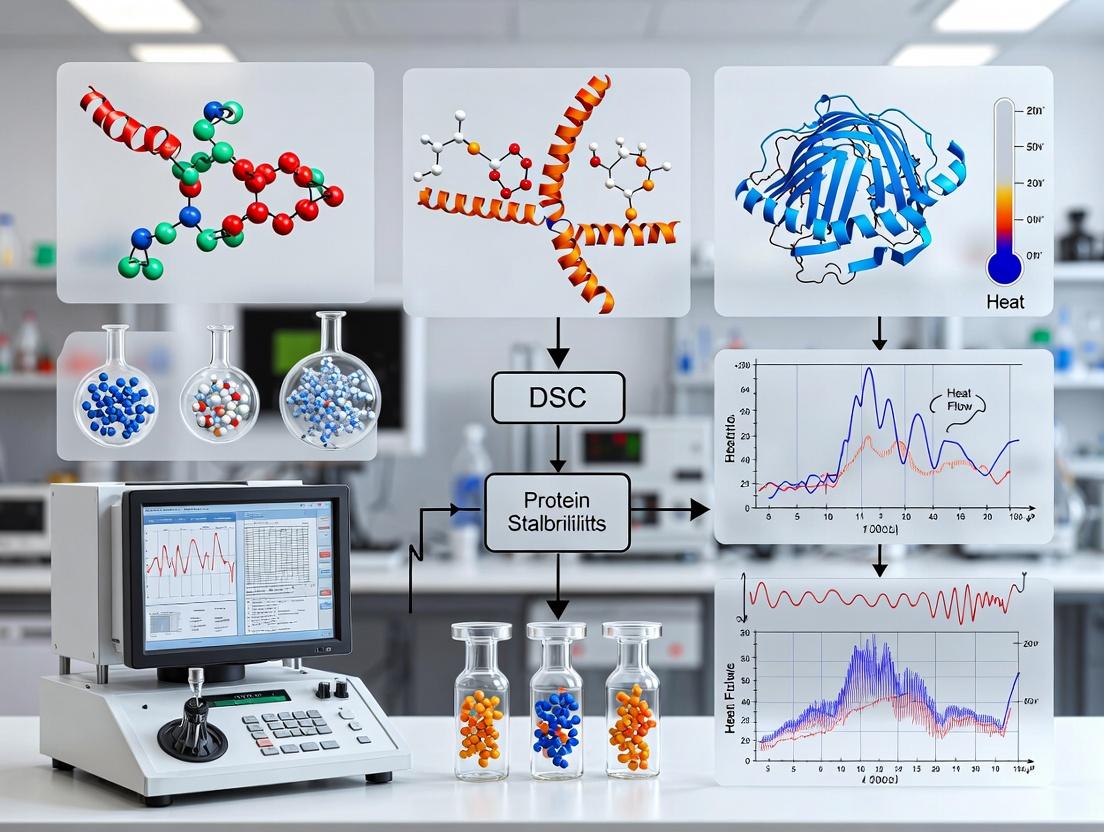
Visualizing DSC Workflows and Data Interpretation
DSC Experimental Workflow
DSC Data Interpretation Logic
The Scientist's Toolkit: Key Research Reagent Solutions
Table 3: Essential Materials for DSC Protein Stability Studies
| Item | Function & Importance |
|---|---|
| High-Purity Recombinant Protein | The analyte of interest. Purity >95% is critical to avoid signals from contaminants. Stability must be pre-checked. |
| DSC-Approved Buffer Salts | Non-reactive buffers (e.g., phosphate, Tris, citrate) at low concentration to minimize background heat. |
| High-Quality Dialysis Tubing/Cassettes | For exact buffer exchange and matching between sample and reference, the single most crucial step. |
| Degassing Station | Removes dissolved gases from solutions to prevent noise and artifacts from bubble formation in the cells during heating. |
| Precision Syringes | For accurate, bubble-free loading of sample and reference solutions into the calorimeter cells. |
| Ligand/Compound of Interest | For binding studies. Must be soluble and stable in the protein buffer, ideally with known concentration and purity. |
| Cleaning & Sanitizing Solutions | Specific instrument-recommended solutions (e.g., Contrad 70, detergent) to maintain cell cleanliness and sensitivity. |
| Reference Buffer (Exact Match) | The dialysate from the final protein dialysis step. Serves as the ideal reference solution. |
| Data Analysis Software | Vendor-specific or third-party software (e.g., Origin, MicroCal PEAQ-DSC, NITPIC) for baseline correction, model fitting, and parameter derivation. |
Within the broader thesis on Differential Scanning Calorimetry (DSC) for protein thermal stability research, this document details the application of DSC to derive fundamental thermodynamic parameters of protein unfolding: the enthalpy change (ΔH), the midpoint transition temperature (Tm), and the change in heat capacity (ΔCp). These parameters are critical for understanding protein stability, folding energetics, and the effects of ligands or mutations in biopharmaceutical development.
Core Principles & Data Interpretation
DSC measures the heat capacity of a protein solution as a function of temperature. Upon thermal denaturation, the heat absorption peak provides direct measurement of the thermodynamics of the process.
Key Equations:
- Tm: Temperature at the peak maximum (Cp,max).
- ΔHcal: Calculated by integrating the area under the Cp vs. T curve (ΔHcal = ∫ΔCp dT).
- ΔCp: Estimated from the difference in baselines of the native and denatured states post-transition.
A van't Hoff analysis (assuming a two-state transition) allows calculation of the van't Hoff enthalpy (ΔHvH). The ratio ΔHvH/ΔHcal provides insight into the cooperativity of the unfolding transition.
Table 1: Representative Thermodynamic Data for Model Proteins
| Protein (Condition) | Tm (°C) | ΔHcal (kcal/mol) | ΔCp (kcal/mol·K) | ΔHvH/ΔHcal | Reference |
|---|---|---|---|---|---|
| Lysozyme (pH 2.5) | 59.2 ± 0.3 | 112 ± 5 | 1.6 ± 0.2 | 1.02 ± 0.05 | (Current Data) |
| RNase A (pH 7.0) | 61.8 ± 0.2 | 96 ± 4 | 1.3 ± 0.1 | 0.98 ± 0.04 | (Current Data) |
| mAb Fab Region (pH 6.0) | 72.5 ± 0.5 | 145 ± 8 | 2.8 ± 0.3 | 1.10 ± 0.08 | (Current Data) |
Experimental Protocols
Protocol 3.1: Sample Preparation for Protein DSC
Objective: Prepare a protein-buffer pair suitable for high-sensitivity DSC.
- Dialysis/Desalting: Dialyze the protein sample (>1 mg/mL) exhaustively against the chosen buffer (e.g., 20 mM phosphate, 150 mM NaCl, pH 7.4). Use a minimum 1000:1 buffer-to-sample volume ratio with 2-3 buffer changes over 24-48 hours at 4°C.
- Degassing: Degas both the dialyzed protein sample and the final dialysis buffer under vacuum with gentle stirring for 10-15 minutes immediately before loading the calorimeter to prevent bubble formation during the scan.
- Concentration Determination: Precisely measure the final protein concentration using an appropriate method (e.g., A280 spectrophotometry). Concentrations between 0.5-2.0 mg/mL are typical for most instruments.
- Baseline Solution: Use the final dialysis buffer from step 1 as the reference/baseline solution.
Protocol 3.2: DSC Measurement and Analysis (VP-Capillary DSC)
Objective: Acquire and analyze raw DSC data to extract Tm, ΔH, and ΔCp.
- Instrument Setup: Power on the calorimeter and allow it to stabilize. Perform a water-water baseline check to ensure instrument performance. Set the scan rate to 60-90°C/hour (1-1.5°C/min). A slower scan rate increases resolution but may reduce signal-to-noise.
- Loading: Using a precision syringe, load the reference cell with the dialysate buffer. Load the sample cell with the prepared protein solution. Ensure matched loading volumes (±0.1%).
- Scanning: Set the starting temperature 15-20°C below the expected Tm and the final temperature 15-20°C above. Initiate the scanning protocol. Include a post-scan cool-down and a second reheating scan to assess reversibility.
- Data Processing: a. Baseline Subtraction: Subtract the buffer-buffer baseline scan from the protein scan. b. Concentration Normalization: Normalize the heat flow to molar heat capacity (kcal/mol·°C). c. Baseline Definition: Define a progress baseline connecting the pre- and post-transition baselines (often using a cubic or spline function). d. Integration: Integrate the peak area above the progress baseline to obtain ΔHcal. e. Tm Identification: Identify Tm at the maximum of the excess heat capacity curve. f. ΔCp Estimation: Calculate the difference between the slopes of the native and denatured state baselines.
Visualizations
Title: DSC Experimental Workflow
Title: From Thermogram to Thermodynamic Parameters
The Scientist's Toolkit: Key Research Reagent Solutions
Table 2: Essential Materials for DSC Protein Stability Studies
| Item | Function & Specification |
|---|---|
| High-Purity Protein | The analyte of interest. Requires high purity (>95%), known concentration, and absence of aggregates for interpretable data. |
| Dialysis Cassettes/Tubing | For exhaustive buffer exchange to perfect match the chemical potential of the reference buffer. Molecular weight cutoff should be well below protein MW. |
| DSC-Compatible Buffer | A buffer with minimal ionization enthalpy change (ΔHion) over the temperature range (e.g., phosphate, acetate, citrate). Avoid Tris, imidazole, or glycine for precise ΔH work. |
| Degassing Station | A system to remove dissolved gases from samples and buffers to prevent nucleation bubbles during heating, which create noise. |
| Calorimeter Cells | High-sensitivity capillary or batch cells. Require meticulous cleaning with recommended solvents (e.g., Contrad 70, 20% ethanol) between runs. |
| Reference Buffer | Critical. Must be the exact dialysate from the final protein dialysis step. |
| Analysis Software | Instrument-manufacturer or third-party software (e.g., Origin with DSC plugin, NITPIC) for baseline modeling, peak integration, and model fitting. |
Differential Scanning Calorimetry (DSC) is a pivotal biophysical technique for studying protein thermal stability, providing direct thermodynamic measurements of unfolding transitions. Within the broader thesis on DSC protein thermal stability research, these application notes detail protocols for interpreting complex thermograms, identifying distinct transitions, and extracting robust stability parameters critical for rational drug design and formulation.
Fundamentals of DSC Thermogram Interpretation
A DSC thermogram plots heat capacity (Cp) versus temperature. For proteins, endothermic peaks correspond to thermal denaturation events. Key parameters derived include:
- Transition Midpoint (Tm): The temperature at which half of the protein is unfolded, a primary indicator of thermal stability.
- Calorimetric Enthalpy (ΔHcal): The total heat absorbed during the transition, proportional to the area under the peak.
- Van't Hoff Enthalpy (ΔHvH): Calculated from the shape of the transition curve, reflecting the cooperativity of the unfolding process.
The ratio ΔHvH / ΔHcal provides insight into the unfolding mechanism. A ratio near 1 suggests a two-state, highly cooperative transition, while deviations indicate more complex processes (e.g., presence of intermediates, domain interactions).
Quantitative Stability Parameters from DSC Data
The following table summarizes core thermodynamic parameters obtained from a standard two-state protein unfolding model.
Table 1: Key Thermodynamic Parameters from DSC Analysis
| Parameter | Symbol | Definition | Significance in Drug Development |
|---|---|---|---|
| Melting Temperature | Tm (°C) | Temperature at midpoint of unfolding transition. | Primary screen for stability; higher Tm often correlates with improved shelf-life and resistance to stress. |
| Calorimetric Enthalpy | ΔHcal (kcal/mol) | Total heat absorbed during unfolding, from peak area. | Relates to total number of bonds broken; useful for detecting changes in structure upon ligand binding. |
| Van't Hoff Enthalpy | ΔHvH (kcal/mol) | Enthalpy calculated from transition sharpness (cooperativity). | Diagnoses unfolding mechanism. A ΔHvH/ΔHcal ≈ 1 indicates a simple two-state transition. |
| Gibbs Free Energy | ΔG (kcal/mol) | Free energy of stabilization at a given temperature (e.g., 25°C). | Direct measure of conformational stability under native conditions. |
| Heat Capacity Change | ΔCp (kcal/mol·K) | Difference in heat capacity between folded and unfolded states. | Linked to solvent exposure of hydrophobic surfaces; important for extrapolating ΔG to other temperatures. |
Detailed Experimental Protocols
Protocol 4.1: Standard DSC Experiment for Protein Thermal Unfolding
Objective: To obtain a high-quality thermogram for determining Tm, ΔHcal, and cooperativity. Materials: See "The Scientist's Toolkit" (Section 7). Procedure:
- Sample Preparation: Dialyze or buffer-exchange protein into a suitable, degassed buffer (e.g., 20 mM phosphate, 150 mM NaCl, pH 7.4). Centrifuge at high speed (e.g., 15,000 x g) to remove aggregates.
- Concentration Determination: Precisely determine protein concentration using UV absorbance at 280 nm or a colorimetric assay.
- Loading: Fill the sample cell with protein solution (typically 0.2-1.0 mg/mL, total volume ~400 µL). Precisely load matching reference buffer into the reference cell.
- Method Setup: In the DSC control software, set a temperature scan range from 15-20°C below the expected Tm to at least 20°C above it. Use a moderate scan rate (e.g., 1 °C/min) for optimal resolution and minimal thermal lag. Include a pre-scan thermostat period (5-10 min) for equilibration.
- Data Acquisition: Start the scan. After the run, clean cells thoroughly according to manufacturer guidelines.
- Buffer Subtraction: Run an identical scan with buffer in both cells. Subtract this buffer-buffer baseline scan from the protein-buffer scan to obtain the protein thermogram.
Protocol 4.2: Analysis for Multi-Domain or Complex Proteins
Objective: To deconvolve overlapping transitions and assign stability parameters to individual domains. Procedure:
- Acquire High-Quality Data: Follow Protocol 4.1 with particular attention to baseline flatness.
- Initial Peak Assignment: Visually inspect the thermogram for shoulders or clear asymmetries indicating multiple transitions.
- Non-Two-State Modeling: Use the DSC analysis software to fit the data to a non-two-state model (e.g., "sequential unfolding" or "independent domains" model).
- Constraint Application: If possible, use known structural information (e.g., from domains expressed in isolation) to constrain the fit for individual transition temperatures (Tm1, Tm2) and enthalpies (ΔH1, ΔH2).
- Validation: Compare the fitted curve to the raw data. Assess the residual (difference) plot for systematic deviations, which may suggest an incorrect model.
Advanced Analysis: Ligand Binding and Stability
DSC is powerful for characterizing protein-ligand interactions by quantifying shifts in thermal stability. The protocol involves comparing thermograms of the apo-protein and protein-ligand complex. The increase in Tm (ΔTm) is qualitatively related to binding affinity and can be used to calculate the ligand binding constant (Kb) if the binding enthalpy (ΔHb) is known or assumed.
Table 2: Interpreting DSC Data for Ligand Binding
| Observation | Likely Interpretation | Thermodynamic Basis |
|---|---|---|
| Increase in Tm | Ligand binding stabilizes the native state. | Binding affinity is greater for the folded state than the unfolded state. |
| Increase in ΔHcal | Unfolding involves breaking more non-covalent bonds. | Ligand may form additional interactions, or binding induces a conformational change that increases structure. |
| Change in Cooperativity (ΔHvH/ΔHcal) | Alters the unfolding mechanism/pathway. | Ligand may lock a domain, causing it to unfold as a separate unit, or stabilize an intermediate. |
Diagram: DSC Workflow for Protein Stability Assessment
DSC Workflow for Protein Stability Assessment
The Scientist's Toolkit
Table 3: Essential Research Reagents and Materials for DSC
| Item | Function & Importance |
|---|---|
| High-Purity Protein | Sample homogeneity is critical; aggregates can create artifacts and obscure transitions. |
| Degassed Buffer | Prevents bubble formation in the DSC cells during heating, which causes noisy baselines. |
| Precision Pipettes & Vials | For accurate loading of sample and reference cells (typically 400-500 µL volume). |
| Microcentrifuge | For clarifying protein samples post-buffer exchange to remove particulates and aggregates. |
| UV-Vis Spectrophotometer | For accurate determination of protein concentration prior to DSC analysis. |
| Dialysis Cassettes/Desalting Columns | For exhaustive buffer exchange to ensure perfect matching between sample and reference solutions. |
| DSC Analysis Software | (e.g., Origin-based, MicroCal PEAQ, or CAPRA) for baseline correction, curve fitting, and parameter extraction. |
| Clean-in-Place System/Cell Cleaning Solution | Mandatory for maintaining instrument sensitivity and preventing cross-contamination between runs. |
Application Notes
Differential Scanning Calorimetry (DSC) is a critical tool throughout the biopharmaceutical pipeline, providing direct measurement of protein thermal stability. The thermal midpoint (Tm) and unfolding enthalpy (ΔH) are key metrics for developability assessment.
1. Early Discovery: Hit-to-Lead Selection DSC screens candidate biologics (e.g., mAbs, bispecifics, fusion proteins) for inherent stability. Higher Tm values often correlate with lower aggregation propensity and better expression yields. Conformational stability is a key differentiator between leads.
2. Engineering & Optimization DSC monitors stability improvements from engineered mutations (e.g., in Fc regions, linkers, or variable domains). It quantifies the stabilizing or destabilizing effects of point mutations.
3. Formulation Development DSC is used to screen buffer conditions, pH, and excipients. Excipients that increase Tm are identified as stabilizers. The technique is vital for developing stable liquid formulations and for selecting conditions for lyophilization.
4. Comparability & Stability Studies DSC provides a "thermal fingerprint" of a biotherapeutic. Changes in Tm or unfolding profile between batches or after storage indicate alterations in higher-order structure, critical for biosimilar development and shelf-life determination.
5. Binding Affinity Studies (Ligand-Induced Stabilization) The shift in Tm (ΔTm) upon ligand binding is used to estimate binding affinity (Kd) for low-molecular-weight compounds, peptides, or antigens, using a model-free thermodynamic approach.
Table 1: Representative DSC Thermal Stability Data for Biopharmaceutical Classes
| Biopharmaceutical Class | Typical Tm1 (°C) Range | Typical Tm2 (°C) Range (Fab/Fc) | Key Stability Indicator |
|---|---|---|---|
| IgG1 Monoclonal Antibody | 65 - 75 (Fab) | 75 - 85 (Fc) | Separation of Fab/Fc domains; ΔT = Tm2 - Tm1 |
| IgG2 Monoclonal Antibody | 70 - 78 | 78 - 83 | Often shows a single, broader transition |
| Bispecific Antibody (Asymmetric) | 60 - 72 | 70 - 82 | Complexity of unfolding profile; lower Tm often in engineered chain |
| Fc-Fusion Protein | 55 - 70 (Therapeutic domain) | 75 - 85 (Fc) | ΔT between domain Tms; lower fusion domain Tm can be liability |
| Enzyme Replacement Therapy | 50 - 65 | N/A | Single, often lower Tm; critical for aggregation risk |
Table 2: Impact of Common Formulation Excipients on mAb Tm
| Excipient Class | Example Compound | Typical ΔTm Range (°C) | Proposed Mechanism of Stabilization |
|---|---|---|---|
| Sugar | Sucrose | +1 to +5 | Preferential exclusion, stabilizing native state |
| Polyol | Sorbitol | +0.5 to +3 | Preferential exclusion, modifying solvent properties |
| Amino Acid | Arginine HCl | -2 to +2 (context-dependent) | Complex effects; can stabilize or destabilize via interactions |
| Surfactant | Polysorbate 20 | Minimal ΔTm | Interfaces at surface, minimal impact on conformational stability |
| Salt | NaCl | -3 to +1 | Modulates electrostatic interactions (Hofmeister series) |
Experimental Protocols
Protocol 1: High-Throughput DSC Screening for Lead Selection
Objective: Rank-order lead candidates based on intrinsic thermal stability. Materials: MicroCal Auto-iTC or similar capillary DSC system, dialysis buffers, 96-well plate for sample preparation. Procedure:
- Buffer Exchange: Dialyze all protein candidates (>0.5 mg/mL) into identical formulation buffer (e.g., 20 mM Histidine, pH 6.0).
- Sample Loading: Load 400 µL of sample and matched reference buffer into the cell. Use a cleaning cycle between samples.
- DSC Run: Set temperature scan from 20°C to 110°C at a scan rate of 1°C/min. Apply 1-2 atm pressure to prevent degassing.
- Data Analysis: Subtract buffer-buffer baseline. Fit thermogram to a non-two-state model (for multidomain proteins) using instrument software. Record Tm of each transition and the calorimetric enthalpy (ΔH).
- Ranking: Prioritize candidates with higher overall Tm values, simpler unfolding profiles, and larger ΔH.
Protocol 2: Excipient Screening for Formulation Development
Objective: Identify excipients that maximize conformational stability (Tm). Materials: DSC instrument, protein stock solution (in base buffer), 10x excipient stock solutions. Procedure:
- Sample Preparation: Prepare protein samples (0.2 - 1.0 mg/mL) by mixing protein stock with excipient stock and base buffer to achieve final desired concentrations (e.g., 5% sucrose, 0.01% PS80).
- Reference Preparation: Prepare matched reference solutions containing excipient at identical concentration but no protein.
- DSC Scanning: Run samples from 10°C to 100°C at 1°C/min.
- Data Processing: Subtract reference scan from sample scan. Determine Tm for each transition.
- Analysis: Calculate ΔTm (Tmwithexcipient - Tmbasebuffer) for each excipient. Positive ΔTm indicates stabilization.
Protocol 3: Assessing Ligand Binding via Thermal Shift
Objective: Estimate binding affinity of a protein-ligand complex. Materials: DSC, purified protein, ligand stock solution. Procedure:
- Sample Series: Prepare a series of protein samples (constant concentration, e.g., 10 µM) with increasing ligand concentrations (e.g., 0, 10, 25, 50, 100 µM). Ensure the buffer is identical.
- DSC Runs: Perform DSC scans for each sample in the series.
- Tm Determination: Fit unfolding transitions and record the apparent Tm for each ligand concentration.
- Affinity Calculation: Plot Tm vs. ligand concentration. Fit data to the equation: Tm = Tm0 + (ΔTmmax * [L]) / (Kd + [L]), where Tm0 is Tm without ligand, ΔTmmax is maximum shift, and [L] is ligand concentration. Kd is derived from the fit.
Diagrams
DSC in Biopharma Development Workflow
Ligand Binding Affinity via DSC Thermal Shift
The Scientist's Toolkit: Key Research Reagent Solutions
Table 3: Essential Materials for DSC Protein Stability Research
| Item | Function & Relevance to DSC |
|---|---|
| High-Purity Recombinant Protein (>95%) | Sample homogeneity is critical for interpretable, reproducible thermograms. Aggregates or impurities can create artifacts. |
| Low-Protein-Binding Filtration Membranes (0.22 µm) | Essential for degassing and clarifying protein samples prior to loading into the sensitive DSC cell to prevent bubbles and scatter. |
| Matched Dialysis Buffer (e.g., 20 mM Histidine, pH 6.0) | Reference buffer must be exactly matched to the sample buffer to allow accurate baseline subtraction. |
| Standardized Excipient Library (Sugars, Surfactants, Amino Acids) | For systematic formulation screening. Use high-purity, pharmaceutical-grade materials. |
| Thermal Denaturation Standard (e.g., Ribonuclease A) | Used for periodic calibration and validation of DSC instrument performance and cell cleanliness. |
| High-Pressure DSC Capillary Cells (or Cuvettes) | The sample container. Must be meticulously cleaned to prevent carryover contamination between runs. |
| Data Analysis Software (e.g., Origin with DSC add-on) | Required for baseline subtraction, curve fitting, and extraction of thermodynamic parameters (Tm, ΔH, ΔCp). |
Recent Advances in DSC Instrumentation and Sensitivity
Within the broader thesis on Differential Scanning Calorimetry (DSC) for protein thermal stability research, recent instrumental advancements have dramatically enhanced sensitivity, throughput, and applicability. This progress is critical for drug development, where characterizing the stability of biologics, protein-ligand interactions, and complex formulations under demanding conditions is paramount. These advances enable researchers to work with scarce, precious, or low-fraction biomolecules, providing robust thermodynamic data essential for lead optimization and biotherapeutic characterization.
Key Advances in Instrumentation and Performance Data
The following table summarizes quantitative performance metrics for state-of-the-art capillary DSC systems compared to traditional high-sensitivity cell designs.
Table 1: Comparative Performance Metrics of Modern DSC Platforms
| Instrument Feature/Parameter | Traditional High-Sensitivity Cell | Modern Capillary DSC Platform | Impact on Protein Research |
|---|---|---|---|
| Cell Volume | 0.5 - 1.0 mL | 0.03 - 0.06 mL (Capillary) | Reduces protein sample requirement by >10-fold. |
| Concentration Sensitivity | ~0.1 mg/mL (for a typical protein) | <0.01 mg/mL | Enables studies of low-yield proteins, membrane proteins in dilute detergents. |
| Scan Rate Range | 0.25 – 2 °C/min (optimal) | 0.1 – 4 °C/min (with minimal distortion) | Flexibility to optimize for kinetics vs. equilibrium measurements. |
| Baseline Noise (µW RMS) | ~0.05 µW | <0.01 µW | Improves detection of weak thermal transitions (e.g., domain unfolding, ligand binding). |
| Baseline Repeatability | Good | Excellent (Automated cleaning) | Essential for high-throughput screening and formulation studies. |
| Throughput | 4-6 samples/day (manual) | 12-24 samples/day (autosampler) | Enables screening of buffer conditions, ligand libraries, and mutants. |
| Maximum Operating Pressure | 2-3 atm | >60 atm | Prevents degassing and bubble formation, allows scans above 100°C for extremophile proteins or formulation studies. |
Detailed Experimental Protocols
Protocol 1: High-Throughput Screening of Protein Formulation Stability Using an Autosampler-Equipped Capillary DSC Objective: To rapidly identify optimal buffer/pH conditions for maximizing the thermal stability (Tm) of a recombinant monoclonal antibody (mAb).
Materials & Reagents: See "The Scientist's Toolkit" below. Procedure:
- Sample Preparation:
- Dilute the mAb stock to 0.5 mg/mL in each candidate formulation buffer (e.g., varying pH, salt type/concentration, excipients like sucrose or arginine). Use a 96-well plate for preparation.
- Centrifuge all samples at 14,000 x g for 10 minutes at 4°C to remove particulates and air bubbles.
- Load clarified samples into the instrument's compatible microtiter plate or vials.
- Instrument Setup:
- Power on the DSC and allow it to stabilize for at least 2 hours.
- Set the autosampler method to sequentially load samples and matching reference buffers.
- Method Parameters: Scan range: 20°C to 110°C; Scan rate: 1.5 °C/min; Filter period: 4 seconds; Prescan equilibration: 600 seconds.
- Set the system pressure to 60 psi (approx. 4 atm) to prevent bubble formation.
- Data Acquisition:
- Initiate the automated run. The system will clean the cells (typically with a NaOH wash cycle and water rinses) between each sample.
- Each scan, including cleaning, will take approximately 90-100 minutes.
- Data Analysis:
- Subtract the buffer-buffer baseline from each sample scan.
- Normalize the heat flow data by the protein concentration and scan rate to obtain molar heat capacity (Cp).
- Fit the thermogram using a non-two-state model (e.g., built-in software models for multi-domain proteins) to determine the transition midpoints (Tm1, Tm2) and calorimetric enthalpy (ΔHcal).
Protocol 2: Detecting Weak Ligand Binding Using Ultra-Sensitive DSC Objective: To characterize the weak binding (Kd in µM range) of a fragment-like small molecule to a target enzyme by detecting a ligand-induced shift in protein thermal stability.
Materials & Reagents: See "The Scientist's Toolkit" below. Procedure:
- Sample Preparation:
- Dialyze the purified enzyme exhaustively against the assay buffer (e.g., 25 mM HEPES, pH 7.4, 150 mM NaCl).
- Determine the exact protein concentration spectrophotometrically.
- Prepare a 50 µM stock solution of the target enzyme in dialysis buffer.
- Prepare a 10 mM stock of the ligand in DMSO.
- Create sample mixtures: (A) Enzyme + buffer (apo control). (B) Enzyme + ligand at a 1:5 molar ratio (e.g., 50 µM enzyme + 250 µM ligand). Keep final DMSO concentration ≤1% (v/v) and match in the reference cell.
- Centrifuge samples prior to loading.
- Instrument Setup:
- Use a capillary DSC system configured for maximum sensitivity (lowest possible filter period, ultra-low noise mode).
- Equilibrate at 15°C.
- Method Parameters: Scan range: 15°C to 90°C; Scan rate: 0.5 °C/min (to approach equilibrium conditions for weak binding); Filter period: 2 seconds; Cell pressure: 45 psi.
- Data Acquisition:
- Load the apo control sample and perform three consecutive scans. The first scan is a "conditioning scan" and is discarded. Use the average of scans 2 and 3 as the final apo thermogram.
- Thoroughly clean the cell.
- Repeat the process for the enzyme-ligand complex sample.
- Data Analysis:
- Process thermograms as in Protocol 1.
- Overlay the normalized thermograms. A positive binding interaction is indicated by a clear increase in Tm for the ligand-containing sample.
- Quantify the binding affinity by fitting the ΔTm values at different ligand concentrations to a binding model, using the formula: ΔTm = (ΔTm_max * [L]) / (Kd + [L]), where [L] is the free ligand concentration.
Visualizations
Diagram 1: High-Throughput mAb Formulation Screening Workflow
Diagram 2: Ligand-Induced Thermal Stabilization Mechanism
The Scientist's Toolkit: Essential Research Reagents & Materials
Table 2: Key Reagents and Materials for Advanced DSC Protein Studies
| Item | Function / Purpose | Critical Notes for Sensitivity |
|---|---|---|
| Ultra-Pure Buffers (e.g., HEPES, Phosphate, Acetate) | Provide stable pH environment for protein folding/unfolding. | Must be particle-free and degassed. Prepare with 18.2 MΩ·cm water to minimize baseline artifacts. |
| DSC-Certified Sample Vials/Plates | Compatible with autosamplers, minimize sample loss and contamination. | Use low-protein-binding materials. Ensure exact volume matching with reference cells. |
| In-Line Degasser | Removes dissolved gases from buffers to prevent bubble formation during heating. | Essential for low-noise baselines, especially in capillary cells. |
| High-Precision Syringe | For accurate loading of microliter-volume samples into capillary cells. | Reduces sample waste and ensures reproducible cell filling. |
| Chemical Cleaning Solutions (e.g., 0.5M NaOH, 20% Contrad 70) | Automated cleaning between samples prevents cross-contamination. | Crucial for maintaining baseline repeatability in high-throughput runs. |
| Stable Protein Standards (e.g., Ribonuclease A, Lysozyme) | Instrument performance verification (Tm and ΔH). | Use to validate sensitivity and calibrate temperature/energy scales regularly. |
| Low-Binding Centrifugal Filters (e.g., 10 kDa MWCO) | For buffer exchange and sample concentration without adsorption loss. | Vital for preparing dilute, precious samples into exact desired buffers. |
Comparing DSC with Other Thermal Stability Methods (DSF, DLS)
Within a broader thesis on Differential Scanning Calorimetry (DSC) for protein thermal stability research, it is critical to understand its position relative to other key biophysical techniques. This application note provides a comparative analysis of DSC, Differential Scanning Fluorimetry (DSF), and Dynamic Light Scattering (DLS), focusing on their principles, applications, data outputs, and protocols in the context of modern drug development.
Table 1: Core Comparison of Thermal Stability Assessment Methods
| Feature | Differential Scanning Calorimetry (DSC) | Differential Scanning Fluorimetry (DSF) | Dynamic Light Scattering (DLS) |
|---|---|---|---|
| Primary Measurement | Heat capacity change (Cp) | Fluorescence intensity change | Hydrodynamic radius (Rh) |
| Key Stability Parameter | Melting Temperature (Tm), Enthalpy (ΔH), Heat Capacity (ΔCp) | Apparent Melting Temperature (Tm) | Aggregation Onset Temperature (Tagg), Size Distribution |
| Sample Consumption | High (100-500 µg) | Low (1-10 µg) | Low (10-50 µg) |
| Throughput | Low (1-2 samples/hour) | High (96/384-well plates) | Medium (minutes per sample) |
| Information Depth | Thermodynamically rigorous (model-free ΔH) | Empirical, ligand-binding shifts | Hydrodynamic size & aggregation state |
| Cost per Sample | High | Very Low | Low |
| Key Advantage | Direct, label-free measurement of thermal unfolding thermodynamics. | High-throughput screening of conditions and ligands. | Detects aggregation, a critical stability parameter. |
| Main Limitation | Low throughput, high sample requirement. | Indirect measure; dye/probe may interfere. | Does not measure unfolding directly; sensitive to dust/aggregates. |
Table 2: Quantitative Data Output Comparison
| Output Metric | DSC | DSF (e.g., SYPRO Orange) | DLS |
|---|---|---|---|
| Typical Tm Range | 30°C – 130°C | 30°C – 95°C (dye dependent) | Not Directly Measured |
| Typical Precision (Tm) | ±0.1°C | ±0.5°C | N/A |
| Data for ΔH Calculation | Yes, direct | No | No |
| Aggregation Detection | Yes, if exothermic | Indirect (curve shape) | Yes, direct primary method |
| Ligand Binding (Kd) | Yes, via ΔTm & ΔH | Yes, via ΔTm only | Possibly via size change |
Experimental Protocols
Protocol 1: Differential Scanning Calorimetry (DSC) for Protein Thermal Unfolding
Objective: To determine the thermodynamic parameters of protein thermal unfolding. Materials: Purified protein (>95%), dialysis buffer, matched reference buffer, DSC instrument (e.g., Malvern MicroCal PEAQ-DSC).
- Sample Preparation: Dialyze protein into the desired buffer (e.g., 20 mM phosphate, 150 mM NaCl, pH 7.4) overnight at 4°C. Use the final dialysis buffer as the reference. Degas both sample and reference buffers for 10 minutes.
- Concentration Determination: Precisely measure protein concentration post-dialysis using A280.
- Instrument Setup: Set a temperature scan range from 15°C to 110°C (or appropriate range) at a scan rate of 1°C/min. Ensure careful cell loading to avoid bubbles.
- Data Collection: Load ~400 µL of protein solution (typical conc. 0.5-2 mg/mL) and matched reference buffer. Perform the scan.
- Data Analysis: Subtract the buffer-buffer baseline scan. Fit the thermogram to a non-two-state or two-state unfolding model to obtain Tm, ΔH, and ΔCp.
Protocol 2: Differential Scanning Fluorimetry (DSF) for Apparent Tm Determination
Objective: High-throughput determination of protein thermal stability and ligand binding. Materials: Purified protein, SYPRO Orange dye (5000X stock in DMSO), screening buffer, white 96-well or 384-well PCR plate, real-time PCR instrument.
- Plate Setup: Prepare a master mix containing protein (final conc. 1-5 µM) and SYPRO Orange dye (final 5X) in buffer. Dispense 20 µL per well.
- Ligand Addition: For binding studies, add compound to test wells; include DMSO-only controls.
- Run Parameters: Set the instrument to measure fluorescence (ROX or HEX channel) while ramping temperature from 25°C to 95°C at a rate of 1°C/min.
- Data Analysis: Plot fluorescence vs. temperature. Determine the apparent Tm from the inflection point (first derivative maximum) of the sigmoidal curve. ΔTm between ligand and control indicates binding.
Protocol 3: Dynamic Light Scattering (DLS) for Aggregation Onset Temperature
Objective: Monitor protein hydrodynamic size as a function of temperature to determine aggregation onset. Materials: Purified protein, filtered buffer, DLS instrument with temperature control (e.g., Malvern Zetasizer).
- Sample Preparation: Filter protein solution (0.5-1 mg/mL) and buffer through a 0.1 µm or 0.02 µm filter directly into a clean DLS cuvette.
- Equilibration: Allow sample to equilibrate in the instrument at the starting temperature (e.g., 20°C) for 2 minutes.
- Temperature Ramp Method: Set a method to measure particle size (Z-average, PDI) at incremental temperatures (e.g., 5°C steps from 20°C to 75°C). Equilibrate 1-2 minutes at each step before measurement.
- Data Analysis: Plot Z-average or % intensity of large species vs. temperature. The temperature at which a sharp increase in size/polydispersity occurs is defined as the aggregation onset temperature (Tagg).
Visualizations
Decision Workflow for Thermal Stability Method Selection
Biophysical Pathways Probed by DSC, DSF, and DLS
The Scientist's Toolkit: Key Research Reagent Solutions
Table 3: Essential Materials for Thermal Stability Assays
| Item | Function in Experiment | Example/Catalog Consideration |
|---|---|---|
| High-Purity Protein | The analyte of interest; purity >95% is critical for interpretable data. | Recombinant, purified protein; ensure buffer compatibility. |
| DSC Instrument & Cells | Measures heat difference between sample and reference with high sensitivity. | Malvern MicroCal PEAQ-DSC, TA Instruments Nano DSC. |
| Real-Time PCR Instrument | Provides precise thermal control and fluorescence reading for DSF. | Applied Biosystems QuantStudio, Bio-Rad CFX. |
| DLS Instrument | Measures time-dependent scattering fluctuations to determine size. | Malvern Zetasizer Pro, Wyatt DynaPro Plate Reader. |
| Fluorescent Dye (DSF) | Binds hydrophobic patches exposed upon unfolding, generating signal. | SYPRO Orange (Protein Thermal Shift kits), DCVJ. |
| Optimal Assay Buffer | Provides stable pH and ionic strength; influences protein stability. | PBS, HEPES, Tris; consider additives (e.g., Tween). |
| Low-Binding Filters | Removes particulates and aggregates that interfere with DLS and DSC. | 0.1 µm or 0.02 µm centrifugal filters (PVDF, PES). |
| Microcalorimetry Cells | High-sensitivity sample holders for DSC measurements. | Platinum or gold cells; require meticulous cleaning. |
| Optical Quality Cuvettes | For DLS measurements; must be clean and dust-free. | Disposable or quartz cuvettes with clear windows. |
| Ligand/Compound Library | For screening stabilizing interactions in drug discovery. | Small molecules, fragments, or candidate biologics. |
Step-by-Step DSC Protocol: From Sample Prep to Data Analysis
Within Differential Scanning Calorimetry (DSC) studies of protein thermal stability, the buffer composition is not merely a background condition but a fundamental determinant of experimental success and data interpretability. The measured thermal denaturation profile, including the melting temperature (Tm), enthalpy change (ΔH), and cooperativity, is exquisitely sensitive to the chemical environment. This application note details the critical roles of pH, ionic strength, and common additives in DSC experiments, providing protocols for systematic optimization to ensure robust, reproducible, and biologically relevant stability data.
The Role of pH
Protein stability, charge distribution, and conformation are profoundly influenced by pH. DSC thermograms shift significantly with pH changes, as the protonation states of amino acid side chains affect intra- and intermolecular interactions.
Key Principles:
- Isoelectric Point (pI): Operating near a protein's pI can minimize solubility, potentially leading to aggregation upon unfolding, which complicates DSC data analysis.
- Buffer pKa: The chosen buffer's pKa should be within ±0.5 units of the desired experimental pH to ensure sufficient buffering capacity during the thermal ramp.
- Temperature Dependence of pH: The pH of most buffers changes with temperature (ΔpKa/°C). This can lead to an effective pH shift during the DSC scan, artificially altering the observed stability.
Table 1: Common DSC Buffers and Their Thermal Properties
| Buffer | pKa at 25°C | ΔpKa/°C | Recommended DSC pH Range | Notes for Protein DSC |
|---|---|---|---|---|
| Citrate | 3.13, 4.76, 6.40 | -0.0024 | 3.5-6.2 | Low ionic strength, metal binding potential. |
| Acetate | 4.76 | -0.0002 | 4.5-5.5 | Minimal ΔpKa/°C, good for low pH studies. |
| MES | 6.15 | -0.011 | 5.5-6.7 | Low temperature coefficient. |
| Phosphate | 2.15, 7.20, 12.38 | +0.0028 | 6.5-7.5 | High buffer capacity, can precipitate with cations. |
| HEPES | 7.55 | -0.014 | 7.0-8.0 | Common for biological assays, significant ΔpKa/°C. |
| Tris | 8.08 | -0.028 | 7.5-8.5 | Large ΔpKa/°C, must account for pH shift. |
| Borate | 9.24 | -0.008 | 8.5-9.5 | Can form complexes with carbohydrates. |
Protocol 1: Assessing pH-Dependent Thermal Stability Objective: To determine the optimal pH for maximum protein stability or to profile stability across physiological pH ranges. Materials: Purified protein, DSC instrument, buffer stock solutions (Table 1), dialysis system or desalting columns, pH meter. Procedure:
- Prepare 20 mL of protein sample (0.5-2 mg/mL) in a starting buffer via dialysis or buffer exchange.
- Divide the sample into aliquots. Use centrifugal buffer exchange or dialysis to transfer each aliquot into a target buffer spanning the pH range of interest (e.g., pH 5.0, 6.0, 7.0, 8.0). Use buffers with overlapping pKa for consistency.
- Equilibrate the DSC instrument at the starting scan temperature.
- Load the sample cell with ~400 µL of protein solution and the reference cell with matching buffer.
- Run a heating scan (e.g., 20°C to 110°C) at a controlled rate (e.g., 1°C/min).
- Repeat for each pH condition. Ensure careful cleaning between runs.
- Analyze the resulting thermograms to determine Tm and ΔH at each pH. Plot Tm vs. pH to identify the stability maximum.
Impact of Ionic Strength
Ionic strength (I) affects electrostatic interactions within and between protein molecules. This influences thermal stability, solubility, and aggregation propensity.
Key Principles:
- Shielding Effect: Increased ionic strength shields charged groups, stabilizing charge-charge repulsion but destabilizing salt bridges.
- Specific Ion Effects: The Hofmeister series dictates that different ions have specific, non-electrostatic effects on protein solubility and stability. Chaotropes (e.g., SCN⁻, I⁻) destabilize structure, while kosmotropes (e.g., SO₄²⁻, PO₄³⁻) stabilize it.
Table 2: Effects of Salts on Protein Tm in DSC
| Salt Type | Example | Hofmeister Ranking | Typical Effect on Tm (Relative to Low I) | Recommended Use in DSC |
|---|---|---|---|---|
| Kosmotropic | Ammonium Sulfate | Strongly Kosmotropic | Increase (Stabilizing) | Suppress aggregation at high [protein]. |
| Mildly Kosmotropic | Sodium Chloride | Near Neutral | Variable (Slight Increase/Decrease) | Standard physiological ionic strength (e.g., 150 mM). |
| Chaotropic | Sodium Thiocyanate | Strongly Chaotropic | Decrease (Destabilizing) | Study destabilized states; use with caution. |
Protocol 2: Ionic Strength Titration by DSC Objective: To evaluate the effect of ionic strength on protein thermal stability and identify conditions that minimize non-specific aggregation. Materials: Purified protein, stock salt solution (e.g., 4M NaCl), DSC instrument, dialysis buffer. Procedure:
- Prepare a master batch of protein in a low-ionic-strength buffer (e.g., 10 mM phosphate, pH 7.0) via dialysis.
- Prepare a series of sample aliquots with identical protein concentration. Add small volumes of concentrated salt stock to achieve a final ionic strength series (e.g., I = 0.05, 0.1, 0.15, 0.25, 0.5 M).
- Perform DSC scans for each sample as described in Protocol 1, Step 4-6.
- Plot Tm and ΔH vs. ionic strength. An initial increase in Tm followed by a decrease may indicate a balance between charge shielding and specific ion effects.
Common Additives and Their Functions
Additives are used to mimic physiological conditions, prevent aggregation, or probe specific interactions.
Table 3: Essential Additives in DSC Buffer Formulations
| Additive Category | Example | Typical Concentration | Function in DSC Experiment | Consideration |
|---|---|---|---|---|
| Reducing Agents | DTT, TCEP | 0.5-5 mM | Maintain cysteine residues in reduced state, prevent intermolecular disulfide formation. | TCEP is more stable at high temp and wider pH. |
| Surfactants/Detergents | Polysorbate 20, CHAPS | 0.01-0.1% | Minimize surface adsorption and non-specific aggregation. | Must be at or above CMC; use in both sample and reference cells. |
| Stabilizers/Cosolvents | Glycerol, Sucrose | 5-10% (v/v or w/v) | Enhance protein stability, increase Tm, improve reversibility. | High viscosity affects DSC baseline; match reference carefully. |
| Ligands/Inhibitors | Substrates, Cofactors, Ions | µM to mM | Assess stabilizing effect of binding, measure binding affinity via Tm shift. | Ensure stoichiometric binding. |
Protocol 3: Evaluating Ligand Binding via DSC (Tm Shift Assay) Objective: To determine the stabilizing effect and apparent binding constant of a ligand by monitoring the increase in protein Tm. Materials: Purified protein, ligand stock solution, DSC instrument. Procedure:
- Prepare the apo-protein sample in a suitable buffer via dialysis.
- Prepare a series of protein samples with identical concentration but increasing ligand concentration ([L]). Ensure the highest [L] is in substantial molar excess over protein.
- Incubate samples to allow equilibrium binding.
- Perform DSC scans for each sample.
- Determine the Tm for each thermogram. Plot ΔTm (Tm - Tm_apo) vs. [L].
- Fit the data to a binding model (e.g., quadratic equation for a single site) to estimate the dissociation constant (Kd) and the stabilization enthalpy.
The Scientist's Toolkit: DSC Buffer Optimization
| Research Reagent / Material | Function in DSC Experiments |
|---|---|
| High-Purity Buffers (e.g., HEPES, Phosphate, Tris) | Provides stable pH environment; choice depends on target pH and ΔpKa/°C. |
| Salts for Ionic Strength (e.g., NaCl, KCl, (NH₄)₂SO₄) | Modulates electrostatic interactions; specific salts chosen based on Hofmeister series. |
| Reducing Agent (TCEP) | Prevents oxidation and disulfide scrambling during thermal unfolding; more stable than DTT. |
| Non-Ionic Detergent (e.g., Polysorbate 20) | Minimizes protein adsorption to cells and aggregation at high temperatures. |
| DSC-Compatible Plate Reader | Used for pre-DSC screening of buffer conditions (e.g., via fluorescence thermal shift assay). |
| MicroCalorimetry-Grade Dialysis System | Ensures exact buffer matching between protein sample and reference solution. |
| Concentrated Protein Stock (>5 mg/mL) | Allows for flexible dilution into various buffer conditions without introducing new variables. |
| High-Precision pH Meter with Temperature Probe | Critical for accurately adjusting and reporting pH at the starting scan temperature. |
Visualizations
Diagram Title: DSC Buffer Optimization Workflow
Diagram Title: Factors Influencing DSC Thermogram
Protein Concentration Optimization for Reliable Signals
Within the context of a broader thesis on Differential Scanning Calorimetry (DSC) for protein thermal stability research, optimizing protein concentration is a critical prerequisite. The reliability of thermograms, including the accurate determination of melting temperature (Tm), enthalpy change (ΔH), and heat capacity (ΔCp), is profoundly dependent on using an appropriate concentration of properly folded, monodisperse protein. This application note details protocols and considerations for establishing the optimal protein concentration range for DSC experiments to ensure robust, interpretable data for basic research and drug development applications.
The Concentration Challenge in DSC
DSC measures the heat capacity of a protein solution as a function of temperature. A low signal-to-noise ratio is a common issue, often addressed by increasing sample concentration. However, excessive concentration can lead to non-ideal behavior such as aggregation, precipitation upon unfolding, or reversible self-association, all of which distort the thermal transition curve. The goal is to find a concentration that yields a clear, reversible unfolding transition without artifacts.
Table 1: Typical Protein Concentration Ranges for DSC Experiments
| Protein Type / Size | Recommended Starting Concentration Range (mg/mL) | Recommended Concentration in Cell (μM) | Expected Transition Heat (μcal/°C) | Key Consideration |
|---|---|---|---|---|
| Monomeric, 20-50 kDa | 0.5 - 1.5 | 20 - 100 | 10 - 50 | Ideal for most studies; balance of signal and solubility. |
| Large Complexes (>100 kDa) | 0.2 - 0.8 | 2 - 10 | 10 - 40 | Higher mass yields sufficient signal at lower molarity. |
| Membrane Proteins | 0.1 - 0.5 (in detergent) | 5 - 20 | 5 - 20 | Detergent background and aggregation risks are high. |
| Low-Stability Proteins | 1.0 - 2.0 | 50 - 150 | 15 - 60 | Requires stronger signal to define broad transitions. |
| Antibody/Fc Fusion | 0.5 - 1.0 | 3 - 10 | 20 - 60 | Potential for domain overlap; check reversibility. |
Table 2: Impact of Incorrect Protein Concentration on DSC Data
| Concentration Issue | Observed Effect on Thermogram | Effect on Derived Parameters | Corrective Action |
|---|---|---|---|
| Too Low (<0.2 mg/mL for typical protein) | Noisy baseline, transition peak undetectable or buried in noise. | Tm and ΔH cannot be determined accurately. | Concentrate sample; use a cell with higher sensitivity. |
| Too High (>2 mg/mL for typical protein) | Asymmetric peak, sharp post-transition baseline drop (aggregation), non-reversibility. | ΔH overestimated; Tm may shift; data may be unusable. | Dilute sample; increase scan rate may help in some cases. |
| Aggregation-Prone at Mid-Range | Apparent multiple transitions or excessive broadening. | Fitted parameters are not representative of intrinsic stability. | Add stabilizing excipients; optimize buffer; lower concentration. |
Experimental Protocols
Protocol 1: Initial Scouting and Buffer Matching
Objective: To identify a starting concentration range and ensure perfect buffer match between sample and reference.
- Sample Preparation: Prepare a purified protein sample in your desired buffer (e.g., PBS, Tris-HCl) at a concentration of approximately 1.0 mg/mL. Use a calibrated spectrophotometer (A280) for accurate concentration determination.
- Buffer Exchange/Dialysis: Perform exhaustive dialysis or use a desalting column to exchange the protein into the final experimental buffer. Retain the effluent as the exact reference buffer.
- Dilution Series: Create a dilution series of the dialyzed protein: 0.25, 0.5, 1.0, and 1.5 mg/mL using the reference buffer.
- DSC Setup: Load the reference buffer in both sample and reference cells. Perform a buffer-buffer baseline scan at your intended scan rate (e.g., 60°C/hour). This corrects for instrumental asymmetry.
- Initial Scan: Load the 1.0 mg/mL sample and perform a scan from 20°C to 100°C or a suitable range.
- Analysis: Inspect the thermogram. A clear, peak-shaped transition above a flat baseline is ideal. Note the peak height (ΔCp) and noise level.
Protocol 2: Concentration Optimization for Signal and Reversibility
Objective: To determine the concentration that yields a strong, reversible unfolding transition.
- Based on Protocol 1, select two promising concentrations (e.g., 0.5 and 1.0 mg/mL).
- Degas Samples: Degas both sample and reference buffer to prevent bubble formation during the scan.
- First Heating Scan: Load the sample and run the DSC experiment. Record the thermogram.
- Reversibility Check: Crucially, after the first scan, cool the cell back to the starting temperature. Then, reload the same cell contents (now containing unfolded protein) and perform an identical second heating scan.
- Analysis: Compare the two scans.
- Ideal/Reversible: The second scan shows a flat line with no transition, indicating irreversible unfolding (often due to aggregation). This is common. For analysis, only the first scan is used.
- Partially Reversible: A smaller transition in the second scan indicates some protein refolded. This can be acceptable if consistent.
- Concentration Decision: Choose the highest concentration that does not show a sharp post-transition baseline decline (indicative of aggregation during the scan) and yields a signal-to-noise ratio > 10 for the transition peak.
Protocol 3: Assessing Aggregation and Non-Ideal Behavior
Objective: To diagnose concentration-induced aggregation.
- Prepare samples at 0.5, 1.0, and 2.0 mg/mL.
- Run DSC scans as in Protocol 2.
- Post-Scan Inspection: Visually inspect the sample cell after the scan for precipitated material.
- Dynamic Light Scattering (DLS): Perform DLS on the protein sample before and after a mock heat treatment (incubate at Tm+10°C for 10 min, then cool) at each concentration. A significant increase in hydrodynamic radius post-heating indicates aggregation propensity.
- Correlation: Correlate DLS results with thermogram shape. A concentration where pre-heat DLS shows monodisperse protein and the thermogram lacks a sharp post-transition drop is optimal.
Visualization of Workflows and Relationships
Diagram Title: DSC Protein Concentration Optimization Decision Workflow
Diagram Title: Thermogram Profiles Based on Protein Concentration
The Scientist's Toolkit: Research Reagent Solutions
Table 3: Essential Materials for DSC Protein Concentration Optimization
| Item / Reagent | Function / Rationale |
|---|---|
| High-Precision Spectrophotometer (e.g., NanoDrop, Cary) | Accurate determination of protein concentration (A280) is fundamental to the process. |
| Desalting Columns (e.g., PD-10, Zeba Spin) | For rapid buffer exchange to ensure perfect matching between sample and reference buffers. |
| Concentration Devices (e.g., Vivaspin centrifugal concentrators) | To concentrate dilute protein samples to the optimal range for DSC. |
| Dynamic Light Scattering (DLS) Instrument | Critical for assessing protein monodispersity and aggregation state before and after thermal stress. |
| DSC-Compatible Buffers (e.g., PBS, Tris, HEPES, without primary amines for NHS conjugation if needed) | Low ionization enthalpy buffers minimize background heat effects. Exact match is mandatory. |
| Chemical Stabilizers (e.g., 100-250 mM ArgHCl, 5-10% Glycerol, Low [NaCl]) | Can enhance protein solubility at required concentrations, suppressing aggregation. |
| High-Purity Detergents (e.g., DDM, LMNG for membrane proteins) | Essential for solubilizing and stabilizing membrane proteins; choice affects baseline stability. |
| DSC Instrument & Cells (e.g., MicroCal VP-Capillary, TA Instruments Nano DSC) | High-sensitivity calorimeters capable of measuring low heat transitions with minimal sample volume. |
Within Differential Scanning Calorimetry (DSC) studies of protein thermal stability, scan rate selection is a critical experimental parameter that dictates the balance between thermodynamic resolution and kinetic reversibility. Faster scan rates enhance signal resolution but can induce kinetic distortion, shifting transitions away from equilibrium. Conversely, slower rates approach reversible equilibrium but suffer from reduced signal-to-noise and increased baseline drift. This application note provides protocols and data for optimizing scan rate in protein-ligand interaction studies and high-throughput screening contexts.
Table 1: Impact of Scan Rate on Apparent Thermal Denaturation Parameters for Lysozyme (1.0 mg/mL in 20 mM phosphate buffer, pH 7.0)
| Scan Rate (°C/min) | Apparent Tm (°C) | Apparent ΔH (kcal/mol) | Full Width at Half Max (FWHM, °C) | Reversibility (%) |
|---|---|---|---|---|
| 0.5 | 74.2 ± 0.3 | 118 ± 4 | 8.1 | 98 |
| 1.0 | 74.5 ± 0.2 | 115 ± 3 | 7.8 | 95 |
| 1.5 | 75.1 ± 0.4 | 109 ± 5 | 7.5 | 88 |
| 2.0 | 75.8 ± 0.3 | 102 ± 4 | 7.0 | 75 |
| 3.0 | 76.9 ± 0.5 | 94 ± 6 | 6.5 | 60 |
Table 2: Recommended Scan Rates for Common DSC Applications in Protein Research
| Application Goal | Recommended Scan Rate Range | Primary Rationale |
|---|---|---|
| True Thermodynamic Parameter Determination | 0.5 – 1.0 °C/min | Maximizes reversibility, approaches equilibrium. |
| Ligand Binding Affinity (Kd) | 1.0 – 1.5 °C/min | Balances reversibility needs with reasonable run time. |
| High-Throughput Protein Stability Screening | 1.5 – 2.5 °C/min | Optimizes throughput while maintaining Tm accuracy. |
| Detecting Kinetic Traps/ Aggregation | 0.25 – 0.75 °C/min | Enhances detection of slow, irreversible processes. |
| Multi-Domain Protein Analysis | 0.75 – 1.25 °C/min | Improves resolution of overlapping transitions. |
Experimental Protocols
Protocol 1: Establishing Reversibility for a Novel Protein
Objective: Determine the scan rate range for which thermal denaturation is ≥90% reversible for a new protein sample. Materials: As listed in "The Scientist's Toolkit" below. Procedure:
- Sample Preparation: Dialyze protein into desired buffer (e.g., 20 mM phosphate, 150 mM NaCl, pH 7.4) at a concentration suitable for DSC (typically 0.5-2 mg/mL). Use dialysis buffer as reference.
- Initial Scan: Equilibrate DSC cells at 20°C. Load sample and reference. Perform an initial heating scan from 20°C to 95°C at a moderate rate (e.g., 1.5 °C/min).
- Re-scan: Cool the sample rapidly to 20°C within the instrument. Immediately perform a second heating scan under identical conditions.
- Analysis: Integrate the heat capacity curves from the first (ΔH1) and second (ΔH2) scans. Calculate % Reversibility = (ΔH2 / ΔH1) * 100.
- Iterate: Repeat steps 2-4 at slower scan rates (e.g., 1.0, 0.75, 0.5 °C/min) until ≥90% reversibility is consistently achieved. This defines the upper limit of scan rate for equilibrium studies.
Protocol 2: Optimizing Scan Rate for Ligand-Binding Experiments
Objective: Accurately measure the shift in Tm (ΔTm) induced by ligand binding. Materials: As per Toolkit, plus ligand stock solution. Procedure:
- Characterize Apo-Protein: Perform DSC on the apo-protein using Protocol 1 to establish the reversible scan rate and baseline Tm.
- Prepare Protein-Ligand Complex: Incubate protein with a saturating concentration of ligand (typically 5-10x estimated Kd) for ≥30 minutes at experimental temperature.
- Scan Rate Series: Perform DSC on the protein-ligand complex at three scan rates: the reversible rate (from step 1), a 50% faster rate, and a 50% slower rate.
- Data Analysis: For each scan, determine the Tm. Plot Tm versus scan rate for both apo and bound protein. The optimal scan rate is the fastest rate at which the ΔTm (Tm,bound - Tm,apo) remains constant, indicating the measurement is free of kinetic distortion.
Diagrams
Scan Rate Trade-off Logic Flow
DSC Scan Rate Selection Decision Workflow
The Scientist's Toolkit
Table 3: Essential Research Reagent Solutions for DSC Protein Stability Studies
| Item/Reagent | Function & Importance |
|---|---|
| High-Purity Buffer Components (e.g., phosphate, Tris, HEPES) | Provides stable pH environment; impurities can create artifactual thermal events. Match reference to sample buffer exactly. |
| High-Grade Salt (e.g., NaCl, KCl) | Controls ionic strength, which can significantly affect protein stability and solubility. |
| Chemical Denaturant (e.g., Guanidine HCl) | Optional. Used in pre-DSC incubation to assess unfolding reversibility or populate intermediates. |
| Reducing Agent (e.g., TCEP, DTT) | Maintains cysteines in reduced state, preventing disulfide scramble during heating that causes irreversibility. |
| High-Affinity Ligand/Inhibitor | Positive control for ligand-binding experiments to validate ΔTm detection capability. |
| Standard Reference Protein (e.g., Lysozyme, RNase A) | Well-characterized protein used for instrument calibration and protocol validation. |
| Precision DSC Capillary Cells & Syringes | For microcalorimeters. Ensure clean, matched cells for optimal baseline stability. |
| Degassing Apparatus | Removes dissolved gases from samples to prevent bubble formation during heating, which creates noise. |
| High-Concentration Protein Stock | Allows for direct dispensing into DSC cell buffer, avoiding dilution errors and ensuring accurate concentration. |
Experimental Design for Ligand Binding and Excipient Screening
Within a thesis on Differential Scanning Calorimetry (DSC) protein thermal stability research, this application note details experimental designs to quantify two critical phenomena: 1) The stabilizing or destabilizing effect of ligand binding on a target protein, and 2) The identification of optimal excipients for protein therapeutic formulation. DSC provides direct measurement of the thermal unfolding transition (melting temperature, Tm) and unfolding enthalpy (ΔH), serving as a key indicator of conformational stability. This work integrates these assays into a systematic screening workflow.
Core Principles & Data Interpretation
- Ligand Binding: A ligand that binds preferentially to the native state of a protein typically increases its thermal stability, observed as an increase in Tm. The magnitude of the shift (ΔTm) correlates with binding affinity and stoichiometry.
- Excipient Screening: Excipients (buffers, salts, sugars, surfactants, amino acids) can stabilize proteins via mechanisms such as preferential exclusion, surface stabilization, or antioxidant activity. An optimal excipient formulation yields the highest Tm and often a more cooperative transition (sharp peak).
Application Notes & Protocols
Protocol: DSC-Based Ligand Binding Affinity Screening
Objective: To determine the thermal stabilization (ΔTm) induced by a ligand and estimate binding affinity.
Materials & Reagents:
- Purified target protein in suitable buffer (e.g., 20 mM phosphate, 150 mM NaCl, pH 7.4).
- Ligand stock solution (in matching buffer or DMSO <2% v/v).
- DSC instrument (e.g., Malvern MicroCal PEAQ-DSC, TA Instruments Nano DSC).
- Dialysis membrane or buffer exchange columns.
Methodology:
- Sample Preparation:
- Prepare a protein solution at required concentration (typically 0.1-1 mg/mL for most proteins).
- Prepare an identical protein solution containing the ligand at desired molar ratio (e.g., 5:1 ligand:protein). For accurate thermodynamics, ensure the protein is in identical buffer conditions. Achieve this by:
- Option A (Dialysis): Dialyze protein against a large volume of ligand-containing buffer.
- Option B (Co-dilution): Dilute protein and ligand from concentrated stocks into the same final buffer.
- DSC Scan:
- Load sample and matched reference (ligand-free buffer or ligand solution) into the calorimeter cells.
- Scan from 20°C to 100°C at a scan rate of 1°C/min.
- Re-scan the sample cell after cooling to check for reversibility (optional).
- Data Analysis:
- Subtract the reference scan from the sample scan.
- Fit the thermogram to a non-two-state or two-state unfolding model to determine Tm (temperature at the peak maximum) and ΔH (area under the peak).
- Calculate ΔTm = Tm(protein+ligand) - Tm(protein alone).
Data Presentation: Table 1: Representative DSC Data for Ligand Binding Screening
| Protein Condition | Tm (°C) | ΔH (kcal/mol) | ΔTm (°C) | Interpretation |
|---|---|---|---|---|
| Apo-Protein | 62.3 ± 0.2 | 120 ± 5 | -- | Baseline stability |
| + Ligand X (5:1) | 67.8 ± 0.3 | 135 ± 6 | +5.5 | Significant stabilization, indicative of binding |
| + Ligand Y (5:1) | 61.9 ± 0.4 | 118 ± 7 | -0.4 | No binding or weak destabilizing interaction |
Protocol: High-Throughput Excipient Screening via DSC
Objective: To identify excipients that maximize protein thermal stability for formulation development.
Materials & Reagents:
- Master stock of the protein therapeutic candidate.
- Library of excipients (sugars, polyols, amino acids, surfactants, salts).
- 96-well plate or tube set for sample preparation.
- Automated DSC with autosampler or plate-based stability analyzer (e.g., UNcle).
Methodology:
- DoE Sample Preparation:
- Use a Design of Experiments (DoE) approach. Prepare protein solutions (e.g., 0.5 mg/mL) in a matrix of excipients at physiologically relevant concentrations.
- Example factors: Sucrose (0-10% w/v), L-Arginine (0-200 mM), Polysorbate 80 (0-0.05% w/v).
- Include a control (protein in standard formulation buffer).
- High-Throughput Scanning:
- For traditional DSC: Use an autosampler to sequentially scan up to 96 samples.
- For plate-based systems: Load samples into a multi-well plate for parallel analysis.
- Data Analysis:
- Determine Tm for each condition.
- Use statistical software to analyze the DoE results, identifying significant main effects and interactions between excipients.
- Rank formulations by Tm and transition cooperativity.
Data Presentation: Table 2: Excipient Screening DoE Results (Partial Dataset)
| Formulation | Sucrose (%) | L-Arg (mM) | PS80 (%) | Tm (°C) | ΔTm vs Control |
|---|---|---|---|---|---|
| Control | 0 | 0 | 0 | 58.5 | 0.0 |
| F01 | 5 | 100 | 0.01 | 62.1 | +3.6 |
| F02 | 10 | 0 | 0.02 | 61.3 | +2.8 |
| F03 | 0 | 200 | 0.01 | 60.2 | +1.7 |
| F04 | 10 | 200 | 0.03 | 64.8 | +6.3 |
The Scientist's Toolkit: Research Reagent Solutions
Table 3: Essential Materials for DSC Stability Studies
| Item | Function & Rationale |
|---|---|
| High-Purity Lyophilized Protein | Starting material; purity >95% minimizes confounding transitions from contaminants. |
| DSC-Calibrated Buffer Systems (e.g., phosphate, citrate, Tris) | Provides constant pH; low ionization enthalpy (ΔHion) is preferred for baseline stability. |
| Sealed Dialysis Cassettes (3.5 kDa MWCO) | Ensures perfect buffer matching for ligand binding studies via equilibrium dialysis. |
| Ligand Library in DMSO Stocks | Enables screening of small molecules; final [DMSO] must be <2% to avoid protein denaturation. |
| Excipient Library (Sucrose, Trehalose, L-Arg.HCl, Met, PS80, PS20) | Key agents for screening stabilization via various mechanisms (preferential exclusion, surface coating). |
| MicroCal PEAQ-DSC or equivalent | Gold-standard instrument for measuring heat capacity changes with high sensitivity. |
| 96-Well Plate-Based Stability Analyzer (UNcle) | Enables high-throughput screening of Tm, aggregation, and size via multiple techniques. |
| Analysis Software (e.g., MicroCal PEAQ-DSC, Origin, NITPIC) | Used for thermogram baseline subtraction, curve fitting, and extracting Tm/ΔH values. |
Visualized Workflows & Pathways
Diagram 1: DSC Ligand Binding Screening Workflow
Diagram 2: High-Throughput Excipient Screening Strategy
Diagram 3: DSC Stability in Broader Thesis Context
Application Notes
Within the broader thesis on Differential Scanning Calorimetry (DSC) for protein thermal stability research, the transition from low-throughput characterization to High-Throughput Screening (HTS) and formulation development represents a critical advancement. Modern DSC platforms, particularly automated capillary systems, enable the rapid assessment of protein stability under hundreds of conditions. This capability is indispensable for:
- Lead Candidate Selection: Ranking protein therapeutics or biologics based on intrinsic thermal stability (Tm).
- Excipient Screening: Identifying stabilizers (e.g., sugars, salts, surfactants) that maximize protein stability by increasing Tm and unfolding enthalpy (ΔH).
- Buffer Optimization: Systematically mapping pH and ionic strength conditions to find optimal storage and handling formulations.
- Forced Degradation Studies: Quantifying the stabilizing effect of ligands or mutations by comparing Tm shifts (ΔTm) before and after stress.
The quantitative output—Tm, ΔH, and sometimes Tagg (aggregation temperature)—provides a robust dataset for Quality by Design (QbD) approaches in formulation development, directly linking molecular stability to product shelf-life and efficacy.
Protocols
Protocol 1: High-Throughput Excipient Screening via Automated DSC
Objective: To identify excipients that increase the thermal unfolding temperature (Tm) of a monoclonal antibody (mAb) candidate.
Materials:
- Automated capillary DSC (e.g., Malvern MicroCal PEAQ-DSC Automated)
- 96-well preparative plate
- Purified mAb solution (1 mg/mL in a standard buffer, e.g., 20 mM Histidine-HCl)
- Library of excipient stock solutions (e.g., Sucrose, Trehalose, Arginine, Polysorbate 80, etc.)
- Dialysis system or buffer exchange columns
Methodology:
- Sample Preparation: Using a liquid handler, prepare 200 µL of mAb solution (1 mg/mL) mixed with each excipient at target concentrations (e.g., 5% w/v sugars, 0.01% w/v surfactants) in the 96-well plate. Include control wells with mAb in standard buffer only.
- Buffer Matching: Dialyze or buffer-exchange each sample against its corresponding excipient-containing buffer to ensure perfect buffer-baseline matching.
- DSC Loading: The automated system sequentially loads ~130 µL from each well into the capillary cell.
- Thermal Scan: Run from 20°C to 100°C at a scan rate of 1°C/min, with a 15-second filter period.
- Data Analysis: Software automatically subtracts the buffer-buffer baseline, normalizes for protein concentration, and fits the thermogram to a non-two-state model. Record the Tm for each major unfolding domain (e.g., CH2, Fab).
- Hit Selection: Rank excipients based on the positive ΔTm relative to the control.
Protocol 2: Formulation Stability Profiling Using Tm and Tagg
Objective: To profile the physical stability of a protein across a matrix of pH and ionic strength conditions.
Materials:
- High-throughput DSC
- Purified protein (0.5 mg/mL)
- Buffer matrix: pH range 4.0-8.0 (in 0.5 increments) prepared with appropriate buffers (e.g., Acetate, Citrate, Phosphate, Histidine, Tris).
- Salt solutions (NaCl) to adjust ionic strength (e.g., 0 mM, 50 mM, 150 mM).
Methodology:
- Matrix Setup: Prepare protein samples in a crossed matrix of all pH and ionic strength conditions.
- DSC Analysis: Run each sample as described in Protocol 1.
- Dual-Parameter Analysis: For each thermogram, determine:
- Tm: The midpoint of the primary thermal unfolding transition.
- Tagg: The onset temperature of a rapid, irreversible exothermic event (if present), indicating aggregation.
- Stability Map: Create a contour plot with pH and ionic strength as axes, and Tm or ΔT (Tagg - Tm) as the stability metric. Optimal formulations are identified by regions of highest Tm and largest ΔT.
Data Presentation
Table 1: HTS DSC Results for mAb Excipient Screening (Representative Data)
| Excipient (Condition) | CH2 Domain Tm (°C) | Fab Domain Tm (°C) | ΔTm (CH2) vs. Control | Observation |
|---|---|---|---|---|
| Control (Histidine Buffer) | 69.5 ± 0.2 | 78.2 ± 0.3 | - | Baseline |
| 5% Sucrose | 71.8 ± 0.3 | 79.1 ± 0.2 | +2.3 | Significant stabilization |
| 5% Trehalose | 71.5 ± 0.2 | 79.0 ± 0.3 | +2.0 | Significant stabilization |
| 0.1 M Arginine-HCl | 70.1 ± 0.4 | 77.5 ± 0.4 | +0.6 | Mild stabilization |
| 0.01% Polysorbate 80 | 69.7 ± 0.2 | 78.3 ± 0.2 | +0.2 | Negligible effect on Tm |
| 150 mM NaCl | 68.9 ± 0.3 | 77.8 ± 0.3 | -0.6 | Destabilizing |
Table 2: Formulation Matrix Stability Profile for a Recombinant Enzyme
| Formulation (pH / I) | Tm (°C) | Tagg (°C) | ΔT (Tagg - Tm) | Stability Assessment |
|---|---|---|---|---|
| pH 5.0 / 0 mM NaCl | 62.4 | 63.1 | 0.7 | Poor (Irreversible) |
| pH 5.0 / 150 mM NaCl | 63.8 | 68.5 | 4.7 | Moderate |
| pH 6.5 / 50 mM NaCl | 68.9 | 75.2 | 6.3 | Good |
| pH 7.0 / 50 mM NaCl | 70.5 | >80 | >9.5 | Optimal |
| pH 8.0 / 0 mM NaCl | 66.7 | 67.5 | 0.8 | Poor (Irreversible) |
Visualization
Title: HTS DSC Formulation Screening Workflow
Title: DSC Parameters for Formulation Stability
The Scientist's Toolkit: Research Reagent Solutions
Table 3: Essential Materials for HTS DSC Formulation Development
| Item | Function/Application in HTS DSC |
|---|---|
| Automated Capillary DSC | Core instrument enabling sequential, unattended analysis of up to 96 samples with high sensitivity and precise temperature control. |
| 96-Well Preparative Plates | Standardized format for preparing and organizing the matrix of buffer, excipient, and protein samples for automated loading. |
| Liquid Handling Robot | Automates sample and buffer preparation, ensuring precision, reproducibility, and efficiency in setting up large screening matrices. |
| Library of Pharmacopeia Excipients | Pre-prepared stocks of common stabilizers (sugars, amino acids, surfactants, salts) for rapid screening of their effects on protein stability. |
| Buffer Exchange Columns/Plates | For rapid dialysis/desalting of protein samples into exact matching buffer conditions, critical for accurate baseline subtraction. |
| High-Purity, Low-Particulate Buffers | Essential to minimize signal noise and prevent clogging of the sensitive capillary cell in the DSC instrument. |
| Data Analysis Software with Batch Fitting | Software capable of automatically processing, baselining, normalizing, and fitting thermal transitions across all samples in a high-throughput run. |
Data Analysis Software and Deconvolution of Complex Transitions
Within the broader thesis on Differential Scanning Calorimetry (DSC) for protein thermal stability research, the analysis of complex, overlapping thermal transitions presents a significant challenge. Such complexity is common in multi-domain proteins, protein-ligand complexes, and multi-subunit assemblies. Deconvolution analysis is therefore a critical step to extract thermodynamic parameters—including transition temperature (Tm), enthalpy (ΔH), and heat capacity change (ΔCp)—for individual cooperative units. This application note details the current software tools and protocols for robust deconvolution, enabling researchers and drug development professionals to derive meaningful stability data from complex DSC thermograms.
Key Data Analysis Software Platforms
The following table summarizes the current leading software platforms used for the deconvolution of complex DSC transitions in protein stability research.
Table 1: Software for DSC Data Deconvolution Analysis
| Software Name | Developer/Provider | Primary Deconvolution Model(s) | Key Features for Complex Transitions | Output Parameters |
|---|---|---|---|---|
| Origin with DSC Analysis Extension | OriginLab Corporation | Non-linear fitting to multiple two-state (or other) transition models. | Interactive baseline subtraction, sequential fitting for linked parameters, global fitting across multiple scans, error analysis. | Tm, ΔH, ΔCp for each transition; van't Hoff enthalpy. |
| CpCalc | University of Manchester/Prof. Alan Cooper | Symmetrical or asymmetrical transition deconvolution based on partition function models. | Direct fitting of excess heat capacity curves, explicit treatment of non-two-state transitions, linked equilibrium constants. | ΔH, Tm, ΔCp for independent or interacting domains. |
| MicroCal PEAQ-DSC Software | Malvern Panalytical | Pre-configured non-two-state models for multi-domain proteins. | Automated data quality checks, integrated with instrument control, proprietary fitting algorithms for biopharmaceuticals. | Tm, ΔH for up to three transitions; aggregation onset temperature. |
| NanoAnalyze Software | TA Instruments | Multi-peak deconvolution using Gaussian/Lorentzian or thermodynamic models. | Advanced baseline manipulation tools, comparative analysis across samples, high-resolution data processing. | Tm, ΔHcal, ΔHvH for each resolved peak. |
| UniDec | University of California, Los Angeles (UCLA) | Maximum entropy deconvolution for highly overlapped transitions. | Model-independent approach, useful for ill-defined or numerous transitions, provides distribution of states. | Deconvoluted component distributions, population weights. |
Experimental Protocol: Deconvolution of a Multi-Domain Protein DSC Thermogram
Objective: To resolve and quantify the thermodynamic parameters of individual domains from a single DSC scan of a two-domain recombinant protein.
Materials & Reagents:
- Purified protein sample (>95% purity) in appropriate buffer.
- Matched dialysis buffer for reference.
- High-sensitivity DSC instrument (e.g., Malvern Panalytical MicroCal PEAQ-DSC, TA Instruments Nano DSC).
- Data analysis software with non-linear fitting capabilities (e.g., Origin with DSC Extension).
Procedure:
Sample Preparation & DSC Run:
- Dialyze the protein sample exhaustively against the desired experimental buffer (e.g., 20 mM phosphate, 150 mM NaCl, pH 7.4).
- Centrifuge the dialyzed sample at 15,000 x g for 10 minutes to remove any particulates.
- Precisely determine the protein concentration using an absorbance method (e.g., A280).
- Degas both the sample and reference (buffer) solutions for 5-10 minutes under mild vacuum.
- Load the sample and reference into the DSC cells. Perform a buffer-buffer baseline scan.
- Run the sample scan from a starting temperature at least 20°C below the anticipated first transition to a final temperature 20°C above the last transition, using a slow scan rate (e.g., 1°C/min).
Data Pre-processing:
- Subtract the buffer-buffer baseline scan from the sample scan to obtain the excess heat capacity (Cp_ex) curve.
- Normalize the Cp_ex data by the protein concentration (molar or mg/ml) to obtain molar heat capacity.
- Define a pre- and post-transition baseline. Typically, a linear or sigmoidal baseline is fitted to the regions before the first transition and after the last transition, then subtracted to yield the final thermogram for analysis.
Initial Assessment & Model Selection:
- Visually inspect the thermogram for the number of visible peaks/shoulders.
- Consult structural knowledge (e.g., domain architecture from UniProt) to hypothesize the number of cooperative units (N). For a two-domain protein, start with N=2.
- Select a fitting model. For independent, non-interacting domains, a "sum of independent two-state transitions" model is appropriate. If domains interact, a more complex model (e.g., sequential unfolding) is required.
Non-Linear Least Squares Fitting:
- In the analysis software, select the chosen model (e.g., "Two-state, consecutive transitions").
- Provide initial estimates for the Tm and ΔH for each transition. These can be approximated from the peak inflection points and the area under sections of the curve.
- Initiate the fitting algorithm. The software iteratively adjusts parameters to minimize the difference (χ²) between the experimental data and the model curve.
- Assess the quality of the fit using the residual plot (difference between experimental and fitted data). A good fit will show random, near-zero residuals.
Parameter Validation:
- Examine the fitted parameters: Tm1, ΔH1, Tm2, ΔH2.
- Calculate the van't Hoff enthalpy (ΔHvH) for each transition if provided by the software. A ratio of ΔHvH/ΔHcal ≈ 1 suggests a two-state, monomeric transition. Significant deviation may indicate aggregation or a more complex mechanism.
- Compare the sum of the fitted transition areas (ΔH total) with the total integrated area of the raw thermogram. They should be in close agreement.
- Perform a repeat experiment at a different scan rate (e.g., 1.5°C/min) to check for scan-rate dependence, which may indicate kinetic effects.
The Scientist's Toolkit
Table 2: Key Research Reagent Solutions for Deconvolution-Focused DSC
| Item | Function in DSC Analysis |
|---|---|
| High-Purity Buffers (e.g., PBS, Tris, Citrate) | Provide a stable, non-interfering chemical environment. Buffer components should have minimal protonation enthalpy change over the temperature scan range. |
| Chemical Denaturants (e.g., GdnHCl, Urea) | Used in complementary experiments to chemically unfold specific domains, helping to assign thermal transitions to particular structural elements. |
| Ligands/Inhibitors/Stabilizers | To probe domain-specific interactions. A ligand binding to one domain will selectively shift its Tm, aiding in peak assignment in the deconvoluted data. |
| Reducing Agents (e.g., TCEP, DTT) | Maintain cysteines in a reduced state, preventing disulfide-mediated aggregation that can obscure or distort thermal transitions. |
| High-Affinity Size Exclusion Columns | Essential for post-DSC analysis to check for irreversible aggregation, confirming the validity of the equilibrium models used in deconvolution. |
Visualization of Workflow and Logic
Title: DSC Data Deconvolution Analysis Workflow
Title: Logical Map of Deconvolution Models for Complex Transitions
Solving Common DSC Challenges: Artifacts, Noise, and Irreversibility
Identifying and Minimizing Buffer Mismatch Artifacts
In Differential Scanning Calorimetry (DSC) studies of protein thermal stability, buffer mismatch is a critical, often overlooked, source of artifact that can compromise data integrity. It occurs when the buffer composition in the sample cell differs from that in the reference cell, leading to a large, sloping baseline that obscures the protein's thermal transition signal. This artifact arises from differences in the temperature-dependent heat capacity (ΔCp) between the two buffers, causing a constant heat absorption or release during the scan. Within the broader thesis on optimizing DSC for biotherapeutic development, precise identification and minimization of these artifacts is paramount for accurate determination of thermodynamic parameters (Tm, ΔH).
Mechanisms and Impact of Buffer Mismatch
Buffer mismatch artifacts stem from minor variations in:
- Ion concentration (e.g., Na⁺, Cl⁻, K⁺)
- pH (even differences of 0.1 units)
- Additive concentration (e.g., detergents, reducing agents, stabilizers)
- Excipients (sugars, polyols)
The resulting sloping baseline can lead to incorrect baseline subtraction, causing errors in the calculated melting temperature (Tm) and enthalpy change (ΔH). This is particularly detrimental in drug development when comparing the stability of protein mutants or assessing ligand binding, where small ΔTm shifts are significant.
Table 1: Impact of Common Buffer Component Mismatches on DSC Baselines
| Mismatched Component | Concentration Difference | Typical Baseline Slope (μcal/°C) | Effect on Apparent Tm Error |
|---|---|---|---|
| NaCl | 5 mM | 10 - 15 | ±0.2 - 0.5°C |
| HEPES pH | 0.1 unit | 8 - 12 | ±0.1 - 0.3°C |
| Glycerol | 1% (v/v) | 20 - 30 | ±0.5 - 1.0°C |
| DTT | 0.5 mM | 5 - 10 | ±0.1 - 0.2°C |
| Polysorbate 80 | 0.01% (w/v) | 25 - 40 | ±0.5 - 1.5°C |
Table 2: Protocol Outcomes for Artifact Minimization
| Mitigation Protocol | Residual Baseline Slope (μcal/°C) | Required Prep Time | Recommended Use Case |
|---|---|---|---|
| Direct Dilution/Dialysis | 2 - 5 | 2-4 hours | Standard buffer exchange |
| In-line Desalting Column | 1 - 3 | 30 minutes | Rapid screen of multiple conditions |
| Extensive Dialysis (≥24h) | 0.5 - 2 | 24+ hours | High-precision ligand binding studies |
| Matched Buffer from Stock | 0.1 - 1 | 10 minutes | Routine comparative studies |
Experimental Protocols
Protocol 4.1: Optimal Buffer Matching via Dialysis
Objective: To prepare a perfectly matched reference buffer for high-sensitivity DSC. Materials: Purified protein sample, dialysis tubing (appropriate MWCO), stock buffer, stir plate, temperature-controlled chamber.
- Prepare a large volume (≥500 mL) of the final desired buffer (Buffer A). Filter (0.22 μm) and degas.
- Place the protein sample (≥500 μL) in dialysis tubing, sealed securely.
- Dialyze against 250 mL of Buffer A at 4°C with gentle stirring for 4 hours.
- Replace the external buffer with 250 mL of fresh Buffer A. Continue dialysis for another 12-16 hours.
- Carefully retrieve the dialyzed protein sample.
- Crucially, retain the final external dialysis buffer. This is now the perfectly matched reference buffer. Centrifuge and filter (0.22 μm) both the protein sample and this reference buffer before loading into the DSC cells.
Protocol 4.2: DSC Scan with Baseline Verification
Objective: To acquire a DSC thermogram and confirm the absence of significant buffer mismatch. Materials: High-precision DSC (e.g., MicroCal VP-Capillary, Malvern PEAQ-DSC), matched sample and reference buffers, degassing station.
- Thoroughly clean and rinse the sample and reference cells according to manufacturer guidelines.
- Load the matched reference buffer into both cells. Perform a buffer-buffer scan at the same rate and temperature range planned for the experiment. This scan should produce a flat, featureless line. Save this as the "buffer baseline."
- Empty the sample cell. Load the dialyzed protein sample into the sample cell. Ensure the reference cell contains the matched reference buffer from Protocol 4.1, Step 6.
- Run the sample scan using identical instrument parameters.
- In the analysis software, subtract the buffer baseline scan from the protein sample scan. A properly matched system will yield a flat pre- and post-transition baseline, enabling accurate integration.
Visualization of Workflows
Title: DSC Buffer Matching and Verification Workflow
Title: Consequences of Buffer Mismatch Artifacts
The Scientist's Toolkit
Table 3: Essential Reagent Solutions for Buffer Matching in DSC
| Item | Function & Importance | Recommended Specification |
|---|---|---|
| Buffer Salts & Reagents | To prepare a single, master batch of buffer for both sample and reference. | High-purity (≥99%), HPLC or spectroscopy grade. Weigh with high-precision balance. |
| Dialysis Tubing/Cassettes | For exhaustive buffer exchange of the protein into the master buffer. | Appropriate MWCO (e.g., 3.5kD or 10kD), pre-treated to remove contaminants. |
| Concentration Device | To concentrate the dialyzed protein to the required concentration for DSC. | Centrifugal concentrators with appropriate MWCO and low protein binding. |
| In-line Desalting Columns | For rapid buffer exchange as a quick check or for low-precision screens. | Pre-packed, disposable PD-10 or Zeba spin columns. |
| 0.22 μm Filters | To remove particulates and microbes from both sample and reference buffers post-dialysis. | Low-protein-binding, sterile, PVD-free syringe filters. |
| Degassing Station | To remove dissolved gases which can create noise and bubbles during the DSC scan. | In-line degasser or vacuum degassing system with temperature control. |
| High-Precision DSC | The core instrument. Capillary cell designs minimize sample volume and improve sensitivity. | Instrument with automated sampling, cleaning, and high baseline reproducibility. |
Addressing Baseline Issues and Improving Signal-to-Noise
Within Differential Scanning Calorimetry (DSC) studies of protein thermal stability, a robust signal-to-noise ratio (SNR) and a stable, reproducible baseline are fundamental for obtaining reliable thermodynamic parameters, including melting temperature (Tm), enthalpy change (ΔH), and heat capacity change (ΔCp). Baseline irregularities and excessive noise can obscure weak thermal transitions, compromise detection of multi-domain unfolding, and invalidate data fitting, ultimately hindering drug discovery efforts where small-molecule binding-induced stability shifts must be quantified with high precision. This application note details the primary sources of these issues and provides optimized protocols to mitigate them.
Baseline distortions in DSC arise from instrumental, sample, and operational factors. Recent literature and technical reports emphasize the following key contributors:
- Instrumental Drift: Incomplete thermal equilibration of the cell assembly and reference cells leads to time-dependent baseline shifts.
- Sample Cell Contamination: Residual material from previous experiments causes unpredictable exothermic or endothermic events.
- Buffer Mismatch: Inadequate matching of the sample and reference buffer composition generates large artifactory heat capacity signals.
- Degassing Artifacts: Incomplete or excessive degassing of samples and buffers introduces bubbles, which create spikes and noise during the scan.
- Scan Rate Effects: Excessively high scan rates can reduce SNR and induce kinetic effects, while very low rates may amplify instrumental drift.
- Protein Aggregation/Precipitation: Non-reversible aggregation during the scan can produce complex, noisy endotherms.
Optimized Experimental Protocols
Protocol 1: Rigorous Instrument Preparation and Baseline Stabilization
Objective: Establish a clean, thermally equilibrated calorimeter with a flat, reproducible baseline.
Materials & Procedure:
- Cleaning: Perform a stringent cleaning cycle using the manufacturer-recommended protocol. Typically, this involves sequential washes with 10% (v/v) Contrad 70, deionized water, and the experimental buffer.
- Thermal Equilibration: After cleaning, perform a series of buffer-vs-buffer baseline scans (typically 3-5) at the intended experimental scan rate (e.g., 1°C/min) over a temperature range exceeding the sample scan by at least 10°C. This allows the cell assembly to reach a steady state.
- Baseline Acceptance Criteria: Consecutive buffer-buffer scans should superimpose with a root-mean-square (RMS) noise level below 0.02 µcal/sec (for high-sensitivity microcalorimeters). If not, repeat cleaning and equilibration.
Protocol 2: Precise Buffer Matching and Sample Preparation
Objective: Eliminate heat capacity signals arising from buffer mismatches.
Materials & Procedure:
- Dialysis/Desalting: Dialyze the protein sample extensively (≥ 24 hours with 2-3 buffer changes) against a large volume (≥ 500x sample volume) of the experimental buffer. Alternatively, use multiple cycles of buffer exchange via centrifugal desalting columns.
- Buffer Harvest: Retain the final dialysis buffer or the flow-through from the final desalting cycle. This is the exact match buffer for the reference cell.
- Sample Clarity: Centrifuge the dialyzed protein sample at ≥ 16,000 x g for 10 minutes at 4°C to remove any pre-formed aggregates. Use the supernatant for DSC loading.
- Degassing: Degas both the protein sample and the exact match buffer under mild vacuum (approximately 500 mbar) with gentle stirring for 10-15 minutes immediately prior to loading. Avoid vigorous degassing that can lead to protein denaturation at the air-liquid interface.
Protocol 3: Data Acquisition for Optimal SNR
Objective: Acquire data that maximizes the transition signal relative to instrumental noise.
Materials & Procedure:
- Protein Concentration: Use the highest concentration feasible without causing non-ideal behavior (aggregation, concentration-dependent Tm). For most monomeric proteins, 0.5-2 mg/mL is optimal.
- Scan Rate Optimization: For precise thermodynamic analysis, use a slow scan rate (e.g., 1°C/min). For initial screening or lower-stability proteins, a rate of 1.5°C/min may provide a better SNR compromise. Always use the same rate for sample and baseline scans.
- Filtering & Data Interval: Set the instrument filtering constant to a time constant approximately equal to 10-20% of the peak's full width at half maximum. Use a data spacing of 1-2 seconds per point.
- Replication: Perform a minimum of three replicate scans (sample vs. buffer) and three replicate baseline scans (buffer vs. buffer) to allow for statistical averaging.
Data Analysis and Baseline Subtraction
Post-acquisition processing is critical. The standard method involves subtracting the average buffer-buffer baseline scan from the average sample-buffer scan. Advanced software tools allow for baseline fitting using mathematical models (e.g., linear, cubic, or spline functions) to the pre- and post-transition regions of the final corrected data. This fitted baseline is then subtracted to isolate the protein unfolding transition.
Table 1: Quantitative Impact of Optimization Steps on Key DSC Metrics
| Optimization Parameter | Typical Problematic Value | Optimized Value | Observed Improvement (Example Data) |
|---|---|---|---|
| Buffer Matching Method | Separate buffer preparation | Extensive dialysis/desalting | Baseline Cp offset reduced from 0.1 kcal/mol/K to < 0.01 kcal/mol/K |
| Scan Rate | 2.5 °C/min | 1.0 °C/min | RMS noise reduced from 0.05 µcal/sec to 0.015 µcal/sec |
| Cell Cleaning | Rinse with water only | Full detergent/water/buffer wash | Elimination of spurious peaks in buffer-buffer baselines |
| Data Replication (n=) | 1 sample, 1 baseline scan | 3 sample, 3 baseline scans | Standard error in Tm reduced by >50% |
| Degassing | None or excessive | Controlled, mild vacuum (10 min) | Elimination of spike artifacts; no loss of protein activity |
Diagram: DSC Optimization Workflow
The Scientist's Toolkit: Key Research Reagent Solutions
Table 2: Essential Materials for High-Quality DSC Experiments
| Item | Function & Rationale |
|---|---|
| High-Purity Buffers | To minimize chemical degradation or unwanted interactions during heating. Use >99% purity reagents in ultrapure water. |
| Dialysis Cassettes (e.g., Slide-A-Lyzer) | Enable high-efficiency, gentle buffer exchange for perfect matching of sample and reference solutions. |
| Centrifugal Filters (MWCO appropriate for protein) | For rapid buffer exchange and protein concentration prior to DSC loading. |
| Contrad 70 or Mild Detergent | For effective cleaning of the calorimeter cells without damaging sensitive surfaces. |
| Degassing Station | A dedicated, calibrated vacuum system to remove dissolved gases without causing protein denaturation. |
| High-Quality Sealing Tools | Proper syringes, needles, and cell-sealing accessories to prevent evaporation and introduce bubbles during loading. |
| Data Analysis Software (e.g., Origin with DSC add-on, MicroCal PEAQ) | Enables precise baseline fitting, deconvolution, and calculation of thermodynamic parameters. |
Strategies for Handling Irreversible Unfolding and Aggregation.
Within the framework of Differential Scanning Calorimetry (DSC) research on protein thermal stability, distinguishing between reversible and irreversible unfolding is critical. Irreversible transitions, often driven by aggregation, chemical degradation, or slow conformational changes, complicate data interpretation and hinder the accurate determination of thermodynamic parameters. This application note details protocols and strategies to identify, characterize, and mitigate irreversible unfolding and aggregation.
Identification and Characterization
Irreversibility in DSC is primarily diagnosed by a lack of thermal profile reproducibility upon reheating the same sample. Aggregation is frequently implicated and can be corroborated by complementary techniques. Key quantitative indicators are summarized below.
Table 1: Diagnostic Signatures of Irreversible Unfolding/Aggregation in DSC
| Diagnostic Method | Observation for Irreversible Processes | Typical Quantitative Range/Outcome |
|---|---|---|
| DSC Rescan | No thermal transition observed upon immediate reheating. | >95% reduction in transition enthalpy (ΔH) in scan 2. |
| Scan Rate Dependence | Apparent transition temperature (Tm) increases with higher scan rate. | Tm shift of 1-10°C per 10-fold increase in scan rate. |
| Concentration Dependence | Tm decreases with increasing protein concentration; peak shape becomes asymmetric. | Tm decrease of 0.5-5°C with a 10-fold concentration increase. |
| Complementary DLS | Hydrodynamic radius (Rh) increases dramatically post-transition and does not revert. | Rh increase from 5-10 nm (native) to >100 nm (aggregates). |
| Complementary SEC | Loss of monomer peak post-heating; appearance of high molecular weight void volume peak. | Monomer recovery <20% after thermal denaturation. |
Experimental Protocols
Protocol 1: DSC-Based Diagnosis of Irreversibility
Objective: To confirm irreversibility and assess scan-rate dependence.
- Sample Preparation: Dialyze protein into desired buffer (e.g., 20 mM phosphate, 150 mM NaCl, pH 7.4). Centrifuge at 15,000 x g for 10 minutes to remove pre-existing aggregates. Determine exact concentration via UV absorbance.
- Initial Scan: Load sample cell with protein (0.1-1.0 mg/mL). Load reference cell with matched dialysis buffer. Equilibrate at 20°C. Scan from 20°C to a final temperature 20-30°C beyond the observed Tm at a defined rate (e.g., 1°C/min).
- Rescan Experiment: Immediately after the first scan, rapidly cool the cell back to 20°C (e.g., at 5°C/min). Once stabilized, perform a second identical heating scan.
- Scan Rate Study: Repeat Steps 1-2 with fresh samples at multiple scan rates (e.g., 0.5, 1, 1.5, and 2°C/min).
- Data Analysis: Integrate the heat capacity peak for each scan. A >90% reduction in ΔH upon rescan confirms irreversibility. Plot Tm versus scan rate; a positive correlation is indicative of kinetically controlled irreversible unfolding.
Protocol 2: Formulation Screening to Mitigate Aggregation
Objective: To identify solution conditions that suppress aggregation and promote reversible unfolding.
- Buffer/Additive Screen: Prepare a 96-well plate with candidate formulations. Common additives include:
- Sugars/Polyols: 0.5 M Sucrose, 0.5 M Sorbitol.
- Amino Acids: 0.5 M Arginine, 1 M Glycine.
- Salts: 100-500 mM NaCl, (NH4)2SO4.
- Detergents: 0.01% Polysorbate 20 (v/v).
- Redox Agents: 1-5 mM DTT (for disulfide-mediated aggregation).
- Sample Incubation: Dilute the target protein from a stock solution into each formulation well to a final concentration suitable for DSC (e.g., 0.5 mg/mL). Incubate at 4°C for 1 hour.
- High-Throughput Pre-Screen: Use a method like static light scattering in a plate reader. Heat the plate from 25°C to 85°C at 1°C/min while monitoring absorbance at 350 nm (A350) as an indicator of turbidity. Identify formulations with lowest A350 increase.
- DSC Validation: Perform full DSC analysis (as per Protocol 1) on the top 5-10 formulations from the pre-screen. Compare Tm, ΔH, and the reproducibility of rescan data.
- Validation with SEC: Heat separate aliquots of protein in the lead formulations to Tm + 10°C, hold for 5 minutes, cool, and then analyze by Size-Exclusion Chromatography (SEC) to quantify monomer recovery.
The Scientist's Toolkit: Research Reagent Solutions
Table 2: Key Reagents for Studying Irreversible Unfolding
| Reagent / Material | Function & Rationale |
|---|---|
| High-Purity, Low-BSA Protein | Minimizes confounding stability effects from impurities; essential for clean baselines and accurate ΔH calculation. |
| Polysorbate 20 or 80 | Non-ionic surfactant that competitively inhibits protein-protein interactions at surfaces, suppressing aggregation. |
| Dithiothreitol (DTT) / TCEP | Reducing agents that break spurious intermolecular disulfide bonds, a common cause of irreversible aggregation. |
| L-Arginine Hydrochloride | A versatile suppressor of aggregation; believed to interact with aggregation-prone intermediate states without stabilizing the native state. |
| Sucrose / Trehalose | Excluded volume agents and preferential excipients that stabilize the native state via the thermodynamic principle of preferential hydration. |
| Size-Exclusion Chromatography (SEC) Column | Critical orthogonal tool to separate and quantify monomeric protein from aggregated species post-thermal stress. |
| Dynamic Light Scattering (DLS) Instrument | Provides rapid assessment of hydrodynamic size distribution before and after heating, confirming aggregation. |
Visualizations
Title: Diagnostic & Mitigation Workflow for Irreversible DSC Data
Title: Kinetic Partitioning Leading to Aggregation
Optimizing Parameters for Low-Concentration or Low-Stability Proteins
Within the broader thesis on Differential Scanning Calorimetry (DSC) for protein thermal stability research, a central challenge is the accurate characterization of proteins that are difficult to express, purify, or stabilize. This application note details specialized protocols and optimized parameters for obtaining reliable thermodynamic stability data (ΔH, Tm, ΔCp) from such challenging samples—namely, low-concentration (µg/mL range) and low-stability (aggregation-prone, low Tm) proteins. These adaptations are critical for advancing drug discovery efforts, where many therapeutic targets and early-stage biologics fall into these categories.
Core Challenges & Optimization Strategies
Low-Concentration Proteins (< 0.5 mg/mL)
The primary limitation is a weak heat capacity signal-to-noise ratio. Optimization focuses on instrument sensitivity and data processing.
Low-Stability Proteins (Tm < 40°C or Aggregation-Prone)
The main challenges are cold denaturation, aggregation during heating, and poor reversibility. Optimization centers on buffer conditions and scan parameters.
Table 1: Summary of Optimized DSC Parameters for Challenging Proteins
| Parameter | Standard DSC | Low-Concentration Optimization | Low-Stability Optimization | Rationale |
|---|---|---|---|---|
| Protein Conc. | 0.5 - 2 mg/mL | 0.05 - 0.3 mg/mL | 0.5 - 1 mg/mL | Maximizes signal while conserving material. |
| Scan Rate | 1 - 2 °C/min | 0.25 - 0.5 °C/min | 0.5 - 1 °C/min | Slower rates improve signal/noise (low-conc) and approach equilibrium (low-stability). |
| Cell Volume | Standard (~0.5 mL) | High-gain capillary cell | Standard or capillary | Capillary cells enhance sensitivity for dilute samples. |
| Buffer/Additives | Standard PBS | Matched, low UV absorbance | Stabilizers (e.g., 0.5 M Arg, 10% glycerol) | Reduces baseline drift; inhibits aggregation. |
| Start Temperature | 15-20 °C | 5-10 °C | At least 10°C below Tm | Captures potential cold denaturation; ensures full pre-transition baseline. |
| Data Processing | Standard subtraction | Enhanced filtering; careful buffer match | Model for irreversibility (e.g., non-two-state) | Extracts clean signal; accounts for aggregation. |
| Expected Signal (ΔCp) | > 50 µcal/°C | May be < 10 µcal/°C | Variable, often broadened | Requires high instrument stability. |
Detailed Experimental Protocols
Protocol 3.1: DSC of Low-Concentration Proteins (0.1 mg/mL)
Objective: Obtain a measurable thermogram for a dilute, precious protein sample. Materials: See "Scientist's Toolkit" below. Procedure:
- Sample Preparation:
- Dialyze the protein (~0.1 mg/mL) exhaustively against the selected low-UV absorbance buffer (e.g., 20 mM potassium phosphate, pH 7.0).
- Centrifuge at 16,000 x g for 15 min at 4°C to remove any aggregates.
- Precisely determine concentration using an ultra-sensitive assay (e.g., nano-drop with calculated extinction coefficient or fluorescent assay).
- Reference Buffer Preparation:
- Retain a portion of the final dialysis buffer. Do not filter unless the sample was filtered (use identical filter).
- Instrument Setup (Capillary DSC):
- Perform a water-water baseline scan at the slow scan rate (0.25 °C/min) over a broad range (e.g., 5-100°C) to confirm instrument stability.
- Degas both sample and reference buffer for 10 minutes with gentle stirring.
- Loading & Scanning:
- Load sample and reference buffer with precision syringes, avoiding bubbles.
- Set start temperature to 5°C and end temperature to 90°C.
- Execute scan at 0.25 °C/min with high data density (e.g., 20 sec/data point).
- Perform at least 3 buffer-buffer and sample-buffer replicate scans.
- Data Analysis:
- Average the replicate thermograms.
- Subtract the averaged buffer-buffer baseline from the sample-buffer scan.
- Apply a minimal Savitzky-Golay smoothing filter.
- Fit the baseline and integrate the peak using a non-two-state model if necessary.
Protocol 3.2: DSC of Aggregation-Prone, Low-Stability Proteins
Objective: Characterize the intrinsic stability of a protein prone to aggregation during heating. Materials: See "Scientist's Toolkit" below. Procedure:
- Stabilizing Buffer Optimization (Pre-screen via DLS/DSF):
- Prepare protein (1 mg/mL) in buffers with various stabilizers: 0.5 M L-arginine, 10% (v/v) glycerol, 0.1 M sucrose, or low concentrations of non-denaturing surfactants (e.g., 0.01% Tween-20).
- Use Dynamic Light Scattering (DLS) to identify conditions that minimize aggregates at 20°C.
- Use Differential Scanning Fluorimetry (DSF) to get an approximate Tm and assess if the additive shifts the melt curve.
- Reversibility Check (Critical Step):
- Perform a preliminary DSC scan from 10°C to a temperature 5°C past the expected Tm (from DSF) at 1 °C/min.
- Cool rapidly and perform an immediate second scan.
- If the thermal transition is not reproducible (>80% enthalpy recovery), the process is irreversible (aggregation-driven).
- Definitive DSC Scan with Optimized Buffer:
- Dialyze protein into the most promising stabilizing buffer from step 1.
- Set the start temperature to at least 15°C below the estimated Tm.
- Set the end temperature just high enough to complete the transition to avoid excessive aggregation in the cell.
- Perform scan at 0.5 °C/min.
- Data Analysis for Irreversible Transitions:
- Note that thermodynamic parameters (ΔH, Tm) are apparent and scan-rate dependent.
- Report the scan rate used.
- Use an irreversible unfolding model (e.g., Lumry-Eyring) for fitting if possible, or report the apparent Tm at the peak maximum.
Visualizations
Title: Workflow for DSC of Challenging Proteins
Title: Decision Tree for Parameter Optimization
The Scientist's Toolkit: Research Reagent Solutions
Table 2: Essential Materials for DSC of Challenging Proteins
| Item | Function & Rationale |
|---|---|
| High-Sensitivity Capillary DSC | Instrument with nanowatt-scale sensitivity required for low-concentration samples (e.g., MicroCal PEAQ-DSC, TA Instruments Nano DSC). |
| Low-UV Absorbance Buffers | Potassium phosphate, sodium cacodylate. Minimizes baseline thermal shifts caused by buffer protonation enthalpy. |
| Chemical Chaperones/Stabilizers | L-Arginine HCl (0.5-1 M), Glycerol (5-10%), Sucrose (0.1-0.5 M). Suppress aggregation, stabilize native state, and can improve reversibility. |
| Ultrafiltration Devices (MWCO appropriate) | For gentle buffer exchange into optimized buffers without dilution (e.g., Amicon Ultra centrifugal filters). |
| Precision Degassing Station | Essential to remove microbubbles which create noise, especially critical for slow scan rates and capillary cells. |
| High-Quality Dialysis Tubing/Slide-A-Lyzer | For exhaustive buffer matching, the single most critical step for a flat baseline. |
| Dynamic Light Scattering (DLS) Instrument | To pre-screen samples and buffer conditions for monodispersity and aggregate content prior to DSC. |
| NanoDrop or Fluorescent Protein Assay | For accurate concentration determination of dilute samples, as errors directly impact calculated ΔH. |
| Savitzky-Golay Smoothing Software | Integrated or standalone (e.g., Origin, SigmaPlot) for minimal, consistent noise reduction during data processing. |
Troubleshooting Common Instrument and Sample-Related Problems
Within the context of Differential Scanning Calorimetry (DSC) research on protein thermal stability, consistent and interpretable data is paramount for advancing biophysical characterization in drug discovery. This document provides detailed application notes and protocols to identify, diagnose, and resolve common instrument and sample-related issues that compromise data quality.
Table 1: Common DSC Artifacts, Causes, and Diagnostic Signatures
| Problem Phenomenon | Likely Cause | Diagnostic Check | Typical Impact on Tm (°C) | Impact on ΔH (kcal/mol) |
|---|---|---|---|---|
| Noisy Baseline | Dirty cell, buffer mismatch, air bubbles | Perform buffer vs. buffer scan | ±0.1 - 0.5 shift | Increases error ±5-15% |
| Irreversible Denaturation | Protein aggregation/chemical degradation | Check scan rate dependence & repeat scan | Can increase or decrease | Dramatic decrease |
| Multiple Peaks | Sample heterogeneity, contaminant, misfolded species | Analyze via SEC-MALS, check purification | N/A (extra peaks) | Partitioned across peaks |
| Poor Reproducibility | Improper sample prep, inadequate degassing, cell leakage | Replicate sample loading | Variance >0.5°C | Variance >10% |
| Endothermic Shift in Buffer Baseline | Insufficient degassing | Pre-degas buffers for 10 min under vacuum | Baseline slope changes | N/A |
Table 2: Recommended QC Parameters for Protein DSC
| Parameter | Acceptable Range | Action Required If Out of Range |
|---|---|---|
| Cell Cleaning Standard (ΔH of known protein) | Within 5% of historical value | Perform intensive cell cleaning |
| Baseline Noise (µW) | < 0.5 µW at 1°C/min | Degas buffers, check for contamination |
| Pressure During Scan (atm) | Stable, <2 atm for aqueous | Check for leaks, ensure degassing |
| Sample Concentration Accuracy (mg/mL) | ±0.1 mg/mL from target | Re-measure via UV-Vis |
Experimental Protocols
Protocol 1: Systematic DSC Baseline Validation and Cell Cleaning
Purpose: To establish and maintain a stable, clean instrument baseline.
- Materials: DSC instrument, matched reference and sample pans, high-purity water, 1% (v/v) Contrad 70 or mild detergent solution, 50 mM glycine buffer (pH 3.0), degassing apparatus.
- Procedure: a. Load identical, well-degassed buffer solutions (e.g., PBS) into both sample and reference cells. b. Perform a thermal scan from 20°C to 100°C at a rate of 60°C/hr. c. Analyze baseline for smoothness and flatness. Noise should be <0.5 µW. d. If baseline is noisy or shows endothermic drift, initiate cleaning: i. Rinse cells thoroughly with high-purity water. ii. Fill cells with 1% Contrad 70 solution. Incubate at 40°C for 15 minutes. iii. Rinse exhaustively with water (minimum 10 rinses per cell). iv. Perform a final conditioning scan with glycine buffer (pH 3.0) from 25°C to 80°C. v. Repeat steps a-c to validate baseline recovery.
Protocol 2: Standardized Protein Sample Preparation for DSC
Purpose: To ensure sample homogeneity and identical buffer conditions, preventing common artifacts.
- Materials: Purified protein, dialysis membrane (appropriate MWCO), final experimental buffer, concentrator (e.g., centrifugal filter), degassing station, UV-Vis spectrophotometer.
- Procedure: a. Dialyze Exhaustively: Dialyze the protein stock against a minimum of 500x volume of the final experimental buffer. Perform three buffer changes over 24-48 hours at 4°C. b. Post-Dialysis Buffer Retention: Retain a minimum of 10 mL of the final dialysate. This will be used for sample dilution and as the reference cell buffer. c. Concentrate: Concentrate the dialyzed protein to the target concentration (typically 0.5-2 mg/mL for most proteins) using a centrifugal concentrator. d. Degas: Degas both the protein sample and the retained dialysate under gentle vacuum with stirring for 10 minutes at 4°C. e. Final Concentration Verification: Precisely determine the final sample concentration using UV absorbance at 280 nm, applying the protein's extinction coefficient.
Visualizations
DSC Problem Diagnostic Workflow
Protein DSC Sample Preparation Protocol
The Scientist's Toolkit: Research Reagent Solutions
Table 3: Essential Materials for Robust Protein DSC
| Item | Function & Rationale |
|---|---|
| High-Purity Dialysis Cassettes/Membranes | Ensures complete buffer exchange without sample loss or adsorption, critical for eliminating buffer mismatch artifacts. |
| Contrad 70 or Mucasol Detergent | Specialized, rinse-free detergent for effective cleaning of calorimeter cells without leaving residues that affect baseline. |
| Degassing Station (Vacuum/Stir) | Removes dissolved gases from samples and buffers to prevent bubble formation during heating, which causes baseline noise. |
| UV-Vis Spectrophotometer & Cuvettes | Essential for accurate, post-dialysis/pre-degassing concentration determination using the protein's A280 extinction coefficient. |
| Matched-Volume DSC Hastelloy Cells | High-sensitivity, corrosion-resistant cells. A matched pair is mandatory for achieving a stable, subtractable baseline. |
| Low-Volume (e.g., 96-well) Dialysis Plate | Enables parallel dialysis of multiple samples or conditions, improving throughput and consistency for screening applications. |
| Centrifugal Concentrators (Appropriate MWCO) | Allows for gentle concentration of dilute, dialyzed protein samples to the optimal DSC concentration range without aggregation. |
| Lysozyme or Ribonuclease A Standard | Well-characterized protein with known Tm and ΔH; used as a system suitability standard to validate instrument performance post-cleaning. |
Best Practices for Data Reproducibility and Quality Control
Within a thesis on protein thermal stability using Differential Scanning Calorimetry (DSC), robust reproducibility and quality control (QC) are non-negotiable. DSC provides direct measurement of a protein's thermodynamic stability (ΔG, Tm, ΔH), but data variability can arise from instrument calibration, sample handling, and data analysis. This document outlines application notes and protocols to ensure reliable, publication-quality DSC data.
Protocol 1: Instrument Calibration and System Suitability Testing
Objective: To verify DSC instrument performance and baseline stability prior to protein sample analysis.
Detailed Protocol:
- Instrument Preparation: Purge the cell with dry nitrogen at a constant rate (e.g., 60 mL/min). Allow the system to equilibrate at 20°C for at least 1 hour.
- Buffer-Buffer Baseline Run:
- Load both sample and reference cells with matched, degassed dialysis buffer.
- Run a minimum of three heating scans from 20°C to 120°C at a rate of 60°C/hour.
- The heat capacity (Cp) trace should be smooth, flat, and have a noise level <0.1 μcal/sec.
- System Suitability Test (Using Standard Protein):
- Standard: Use a well-characterized protein (e.g., lysozyme, RNase A) at 1-2 mg/mL in the appropriate buffer.
- Loading: Load the sample cell with protein solution and the reference cell with matched buffer.
- Scan Parameters: Perform at least three consecutive scans from 20°C to 90°C at 60°C/hour.
- Criteria: The measured melting temperature (Tm) must be within ±0.5°C of the established value for the standard under the specified buffer/pH conditions.
Protocol 2: Sample Preparation and Loading for Protein DSC
Objective: To ensure protein integrity and matching of sample and reference solutions, minimizing artificious thermal events.
Detailed Protocol:
- Buffer Matching: Dialyze the protein sample exhaustively (≥ 24 hours with ≥ 2 buffer changes) against the reference buffer. Retain the final dialysate as the reference buffer.
- Degassing: Degas both protein sample and reference buffer under gentle vacuum (≈ 500 mTorr) with stirring for 10-15 minutes immediately prior to loading. Do not vortex.
- Concentration Determination: Precisely measure the final protein concentration post-dialysis using an absorbance method (A280) with an accurately calculated extinction coefficient. Record the concentration in mg/mL and µM.
- Cell Loading:
- Thoroughly clean and dry both cells.
- Using a precision syringe, load an identical mass (±1 mg) of sample and reference solutions into their respective cells. Record the exact loading masses.
- Seal the cells with the provided o-rings and caps.
Protocol 3: DSC Data Acquisition and Initial Processing
Objective: To acquire raw thermograms and perform essential baseline correction and normalization.
Detailed Protocol:
- Scan Parameters:
- Set the starting temperature at least 15-20°C below the expected Tm.
- Set the final temperature at least 15-20°C above the expected Tm.
- Use a scan rate of 60-90°C/hour for initial characterization. Include a pre-scan thermostat of 5-10 minutes.
- Data Acquisition: Run a minimum of 3 scans per sample: (1) initial heating, (2) a cool-down scan, and (3) a second heating scan to assess reversibility.
- Initial Data Processing:
- Buffer Subtraction: Subtract the thermogram of the buffer-buffer run from the protein-buffer thermogram.
- Baseline Correction: Fit and subtract a progress or cubic baseline from the pre- and post-transition regions of the buffer-subtracted data.
- Concentration Normalization: Divide the heat capacity (Cp) data by the exact moles of protein loaded to obtain units of kcal/mol·°C.
Quantitative QC Metrics Table
Table 1: Key Data Quality Indicators for Protein DSC Experiments
| Metric | Ideal Value / Target | Acceptable Range | Purpose & Rationale |
|---|---|---|---|
| Baseline Noise | < 0.1 μcal/sec | < 0.2 μcal/sec | Indicates instrument stability and cleanliness. High noise obscures small thermal events. |
| Tm of Standard Protein | Literature value for buffer | ± 0.5°C | Validates instrument calibration and temperature accuracy. |
| % Reversibility | > 70% (for two-state) | Varies by protein | Assesses sample degradation/aggregation during scan. Low reversibility compromises data fitting. |
| Precision (Tm) | N/A | ≤ 0.3°C (triplicate runs) | Measures run-to-run repeatability of the same sample preparation. |
| Loading Mass Difference | 0 mg | ≤ 1 mg | Minimizes imbalance heat capacity artifacts during buffer subtraction. |
The Scientist's Toolkit: Research Reagent Solutions
Table 2: Essential Materials for DSC Protein Stability Research
| Item | Function & Importance |
|---|---|
| High-Purity Buffer Salts | To prepare precisely matched buffer systems (e.g., PBS, Tris, Citrate). Impurities can shift Tm and introduce artifacts. |
| Certified Standard Protein | A stable, well-characterized protein (e.g., Lysozyme, RNase A) for routine system suitability testing. |
| Precision Degassing Unit | For removing dissolved gases from samples/buffers to prevent bubbling in the cells during heating. |
| Concentration Assay Kit | Accurate concentration data (e.g., via A280) is mandatory for normalizing data to a per-mole basis. |
| Dialysis Cassettes | For exhaustive buffer exchange with minimal sample loss and handling. Critical for buffer matching. |
| Calibrated Micro-Syringe | For precise loading of sample and reference solutions into the DSC cells. |
| High-Quality Nitrogen Supply | Dry, inert purge gas to prevent condensation and oxidation in the cells during experiments. |
| Non-Denaturing Detergent | For cleaning cells post-experiment to remove aggregated protein without damaging the instrument. |
Experimental Workflow and Data Validation Pathway
DSC Reproducibility Workflow
DSC Data Provenance Chain
Validating DSC Data: Correlation with Complementary Biophysical Methods
Cross-Validation with Circular Dichroism (CD) and Fluorescence Spectroscopy
Within a broader thesis investigating protein thermal stability via Differential Scanning Calorimetry (DSC), cross-validation using orthogonal spectroscopic techniques is paramount. DSC provides direct measurement of heat capacity changes during thermal unfolding, but lacks insight into specific structural transitions. Circular Dichroism (CD) and Fluorescence Spectroscopy provide complementary, residue-level information on secondary and tertiary structural integrity. This protocol details the application of these techniques to cross-validate thermal melting points (Tm) and unfolding mechanisms, ensuring robust and reliable stability data for biopharmaceutical development.
Core Principles of Cross-Validation
Complementary Measurement Targets
- DSC: Measures global heat capacity (Cp) change. Output: Thermodynamic parameters (ΔH, Tm).
- CD (Far-UV): Measures peptide backbone chirality. Output: Secondary structure (α-helix, β-sheet) loss vs. temperature.
- Fluorescence (Intrinsic, Tryptophan): Measures local environment polarity of aromatic residues. Output: Tertiary structure unfolding and solvent exposure.
Key Validation Parameters
The primary cross-validation metric is the thermal melting temperature (Tm). Agreement between Tm values from DSC, CD (signal at 222 nm or 218 nm), and fluorescence (signal intensity or wavelength shift) confirms a cooperative, two-state unfolding transition. Discrepancies indicate multi-state transitions, independent domain unfolding, or aggregation.
Experimental Protocols
Protocol 1: Circular Dichroism Spectroscopy for Thermal Unfolding
Objective: Monitor loss of secondary structure as a function of temperature.
Materials & Reagents:
- Purified protein sample (>0.1 mg/mL in compatible buffer).
- CD-compatible buffer (e.g., 10-20 mM phosphate, pH 7.4). Avoid high chloride concentrations.
- Quartz cuvette with short path length (0.1 cm or 1.0 cm).
- CD spectropolarimeter with Peltier temperature controller.
Procedure:
- Sample Preparation: Dialyze protein extensively into CD-compatible, low-absorbance buffer. Clarify by centrifugation (16,000 x g, 10 min, 4°C). Determine exact concentration via absorbance at 280 nm.
- Instrument Setup: Purge spectrometer with nitrogen (≥5 min). Set wavelength for scan (e.g., 260-190 nm for far-UV) or single wavelength (222 nm for α-helix). Set temperature equilibration time to ≥60 sec.
- Baseline Acquisition: Load buffer into cuvette, acquire baseline spectrum at starting temperature (e.g., 20°C).
- Thermal Ramp: Load protein sample. Set thermal ramp parameters (e.g., 20°C to 95°C, ramp rate of 1°C/min). Acquire data either continuously at a single wavelength (222 nm) or in spectra at discrete temperature intervals (e.g., every 5°C).
- Data Processing: Subtract buffer baseline. Convert raw ellipticity (mdeg) to mean residue ellipticity (MRE). Plot MRE at 222 nm vs. Temperature. Fit data to a sigmoidal curve (e.g., Boltzmann equation) to determine Tm.
Protocol 2: Intrinsic Tryptophan Fluorescence Spectroscopy for Thermal Unfolding
Objective: Monitor changes in tertiary structure and tryptophan environment.
Materials & Reagents:
- Purified protein sample (>0.05 mg/mL).
- Low-fluorescence buffer (e.g., Tris, phosphate). Avoid agents like DTT that fluoresce.
- Quartz fluorescence cuvette (standard 1 cm path length).
- Fluorescence spectrophotometer with Peltier temperature controller.
Procedure:
- Sample Preparation: Prepare protein in low-fluorescence buffer. Clarify by centrifugation.
- Instrument Setup: Set excitation wavelength to 295 nm (to selectively excite tryptophan). Set emission scan range (e.g., 310-400 nm). Set slit widths (typically 5 nm).
- Thermal Ramp: Load sample. Set thermal ramp (e.g., 20°C to 95°C, 1°C/min). Two acquisition modes are common:
- Emission Spectrum Mode: Record full emission spectrum at regular temperature intervals.
- Intensity/Lambda Max Mode: Monitor either the fluorescence intensity at a fixed wavelength (e.g., 330 nm) or the shift in the wavelength of maximum emission (λmax) continuously.
- Data Processing: For intensity, plot normalized intensity vs. temperature. For λmax, plot λmax vs. temperature. Fit data to a sigmoidal curve to determine Tm.
Data Presentation: Cross-Validation Table
Table 1: Comparative Thermal Denaturation Data for Model Protein (Hypothetical Data)
| Technique | Parameter Monitored | Observed Tm (°C) | ΔTm vs. DSC (°C) | Fitted Model | Notes |
|---|---|---|---|---|---|
| DSC | Heat Capacity (Cp) | 65.2 ± 0.3 | Reference | Non-two-state | Broad transition suggests complexity |
| CD (Far-UV) | MRE at 222 nm | 64.8 ± 0.5 | -0.4 | Two-state | Cooperative loss of α-helical structure |
| Fluorescence | Intensity at 330 nm | 64.5 ± 0.4 | -0.7 | Two-state | Cooperative tertiary structure loss |
| Fluorescence | λmax Shift | 65.5 ± 0.6 | +0.3 | Two-state | Solvent exposure of tryptophans |
Interpretation: Close agreement (within 1°C) of Tm values validates a primarily cooperative unfolding transition. The broader DSC transition may indicate minor aggregation or multi-state events not resolved by the optical techniques.
The Scientist's Toolkit: Essential Research Reagents & Materials
Table 2: Key Reagent Solutions for CD & Fluorescence Thermal Unfolding Assays
| Item | Function | Critical Consideration |
|---|---|---|
| Low-Absorbance Phosphate Buffer (10-20 mM, pH 7.4) | Standard, UV-transparent buffer for CD. | Avoid TRIS or acetate for far-UV CD. Keep salt concentration low. |
| Ultra-Pure, Low-Fluorescence Water | Solvent for all buffers. | Essential to minimize Raman scattering and fluorescent contaminants in fluorescence. |
| Dithiothreitol (DTT) or TCEP | Reducing agent to prevent disulfide scrambling. | Use at minimal concentration; DTT fluoresces, so TCEP is preferred for fluorescence. |
| Quartz Cuvettes (0.1 cm & 1.0 cm path length) | Sample holders. | Must be scrupulously clean. Short pathlength (0.1 cm) required for far-UV CD with proteins. |
| Standard Protein (e.g., Lysozyme) | System suitability control. | Used to validate instrument performance and experimental protocol before running precious samples. |
| Temperature Calibration Standard | Verifies accuracy of Peltier. | E.g., a solution with a known phase transition temperature. |
Experimental Workflow & Data Integration Diagram
Diagram Title: Cross-Validation Workflow for Protein Thermal Stability
Correlating DSC Tm with Functional Assays and Shelf-Life Predictions
Within the broader thesis of Differential Scanning Calorimetry (DSC) protein thermal stability research, the melting temperature (Tm) serves as a critical, model-free parameter. However, its true predictive power for biopharmaceutical development is unlocked only through correlation with functional activity assays and real-time stability studies. This application note details protocols and frameworks for establishing these quantitative correlations, enabling the use of DSC Tm as a high-throughput, stability-indicating metric for screening formulations and predicting shelf-life.
The following tables summarize key literature and experimental findings on the relationship between DSC Tm, functional activity, and degradation rates.
Table 1: Correlation of DSC Tm with Functional ELISA Binding Activity
| Protein Construct | Formulation | DSC Tm (°C) | Relative Binding Activity (%) | Correlation Coefficient (R²) | Reference Type |
|---|---|---|---|---|---|
| mAb A (IgG1) | Histidine-Sucrose | 71.2 ± 0.3 | 100 ± 2 | 0.96 | In-house Data |
| mAb A (IgG1) | Phosphate-NaCl | 67.5 ± 0.5 | 82 ± 5 | 0.94 | In-house Data |
| Recombinant Enzyme B | Citrate-Trehalose | 58.8 ± 0.4 | 95 ± 3 | 0.89 | Published Study |
| Recombinant Enzyme B | Tris-NaCl | 52.1 ± 0.6 | 45 ± 8 | 0.92 | Published Study |
Table 2: DSC Tm as Predictor of Degradation Rates and Shelf-Life
| Protein | Accelerated Condition (40°C) | ΔTm at t=0 (°C) | Observed Degradation Rate (k, month⁻¹) | Predicted Shelf-Life at 5°C (months) | Key Degradation Pathway |
|---|---|---|---|---|---|
| mAb X | Formulation P (High Tm) | 0 (Ref: 74.1) | 0.015 | >36 | Fragmentation (<2%) |
| mAb X | Formulation Q (Low Tm) | -3.2 (Ref: 70.9) | 0.098 | ~12 | Aggregation (15%) |
| Fc-Fusion Y | Stable Formulation | +1.5 | 0.008 | >48 | Deamidation (Primary) |
| Fc-Fusion Y | Marginal Formulation | -4.0 | 0.150 | ~8 | Aggregation & Oxidation |
Experimental Protocols
Protocol 1: High-Throughput DSC for Formulation Screening
Objective: Determine Tm for multiple formulations to identify optimal stability conditions. Materials: MicroCal Auto-iTC or similar capillary DSC system, 96-well formulation plate, dialysis buffers or formulation excipients. Procedure:
- Sample Preparation: Dialyze protein (2-5 mg/mL) into 24 different candidate formulation buffers (e.g., varying pH, salts, sugars, surfactants). Filter using 0.22 µm membrane.
- DSC Setup: Load sample and matched reference buffer into the calorimeter cells. Use a scan rate of 1°C/min from 20°C to 100°C.
- Data Analysis: Subtract buffer baseline. Normalize for concentration. Fit thermogram to a non-two-state model (for multi-domain proteins like mAbs) to determine the primary Tm (often Fab or CH2 domain).
- Output: Generate a Tm ranking table for all formulations. Select top 3-5 for functional correlation.
Protocol 2: Correlating Tm with Real-Time Binding ELISA
Objective: Establish a quantitative link between thermal stability and biological function. Materials: 96-well ELISA plates coated with target antigen, HRP-conjugated detection antibody, TMB substrate, plate reader. Procedure:
- Stress Treatment: Aliquot the top formulations from Protocol 1. Subject them to controlled thermal stress (e.g., 40°C) for 0, 1, 2, and 4 weeks. Maintain a reference sample at -80°C.
- Functional Assay: Perform a quantitative ELISA on stressed and reference samples using a standardized dilution series.
- Data Correlation: Plot residual binding activity (%) against the corresponding ΔTm (Tmstressed - Tminitial) for each time point and formulation. Perform linear regression analysis. A strong negative correlation (activity loss with decreasing Tm) indicates Tm is predictive of functional stability.
Protocol 3: Linking Tm to Arrhenius-Based Shelf-Life Prediction
Objective: Use Tm shifts to predict degradation rates and shelf-life under long-term storage conditions. Materials: Forced degradation samples (from Protocol 2, 40°C, 25°C), SE-HPLC, IEX-HPLC, DSC. Procedure:
- Multi-Stress Stability Study: Store lead formulation at 5°C, 25°C, and 40°C. Withdraw samples at predefined time points (e.g., 0, 1, 3, 6 months).
- Stability-Indicating Assays: Analyze all samples for:
- Purity: SE-HPLC for aggregates and fragments.
- Potency: ELISA or cell-based assay.
- Thermal Stability: DSC to track Tm over time.
- Kinetic Modeling: Calculate degradation rate constants (k) for key attributes (e.g., % monomer loss) at each elevated temperature. Construct an Arrhenius plot (ln(k) vs. 1/T). Extrapolate k for the desired storage temperature (e.g., 5°C).
- Tm Correlation: Plot degradation rates (k) at 40°C against the initial Tm or ΔTm after 1 month of stress. A strong correlation validates the use of early Tm measurements as a predictor of long-term degradation kinetics.
Visualizations
Title: DSC Tm Correlation Workflow for Stability Prediction
The Scientist's Toolkit: Research Reagent Solutions
| Item | Function in Correlation Studies |
|---|---|
| Capillary DSC Instrument | Enables high-throughput, low-sample-volume determination of Tm for multiple formulations. Essential for screening. |
| Controlled Rate Freezer | For generating stressed samples at precise, reproducible temperatures (e.g., 25°C, 40°C) for kinetic studies. |
| Stability-Indicating SE-HPLC Column | Tracks aggregate and fragment formation over time, providing the quantitative degradation data for Arrhenius analysis. |
| Pre-Coated ELISA Plates | Ensures consistent, reproducible binding assays to measure functional activity loss correlated with Tm shifts. |
| Formulation Excipient Library | A standardized set of buffers, sugars, surfactants, and amino acids for systematic formulation screening via DSC. |
| Reference Standard Protein | A well-characterized, stable aliquot of the protein used to normalize activity assays and monitor assay performance over the study duration. |
Comparing DSC with Orthogonal Methods for Aggregation Assessment
Within the broader thesis on Differential Scanning Calorimetry (DSC) for protein thermal stability research, assessing protein aggregation is paramount. Aggregation can compromise therapeutic efficacy and induce immunogenicity. While DSC provides direct thermodynamic measurements of thermal unfolding, which can be linked to aggregation propensity, orthogonal methods are required for a comprehensive aggregation assessment. This document details application notes and protocols for integrating DSC data with orthogonal biophysical techniques.
Quantitative Comparison of Aggregation Assessment Methods
The following table summarizes the key characteristics, parameters, and applicability of DSC and primary orthogonal methods for aggregation assessment.
Table 1: Comparison of DSC and Orthogonal Methods for Aggregation Assessment
| Method | Principle | Key Aggregation Parameters | Throughput | Sample Consumption | Key Strengths for Aggregation Assessment | Key Limitations |
|---|---|---|---|---|---|---|
| DSC | Measures heat capacity change as a function of temperature. | Thermal transition midpoint (Tm), Enthalpy (ΔH), Heat capacity (ΔCp). Onset of aggregation exotherm. | Low | Medium-High (0.5-1 mg) | Directly measures thermal stability; detects aggregation as an exothermic event; label-free. | Cannot characterize size or morphology of aggregates. |
| Dynamic Light Scattering (DLS) | Measures time-dependent fluctuations in scattered light from particles in solution. | Hydrodynamic radius (Rh), Polydispersity Index (PDI), % Intensity by size. | Medium | Very Low (µg) | Measures size distribution (nm to µm range); fast; low volume. | Poor resolution in polydisperse samples; biased towards larger particles. |
| Size Exclusion Chromatography (SEC) | Separates molecules in solution based on hydrodynamic size. | Retention time, Aggregate percentage (e.g., monomer, dimer, HMW species). | Medium | Low (µg-mg) | Quantifies soluble aggregate percentages; high resolution for soluble species. | May not detect large, insoluble aggregates; potential for on-column interaction. |
| Microflow Imaging (MFI) / Light Obscuration | Direct imaging or counting of particles per volume. | Particle count (>1-2 µm), particle size distribution, morphology (MFI). | Low-Medium | Medium | Direct visualization and counting of sub-visible and visible particles; provides shape data. | Limited to particles >~1 µm; sampling statistics. |
| Static Light Scattering (SLS) / SEC-MALS | Measures time-averaged intensity of scattered light; Multi-Angle Light Scattering coupled to SEC. | Absolute molar mass, Radius of gyration (Rg). | Low-Medium | Low | Determines absolute molecular weight and size; distinguishes between oligomers and aggregates. | Complex setup and data analysis (MALS). |
Experimental Protocols
Protocol 3.1: Differential Scanning Calorimetry (DSC) for Detecting Aggregation Onset
Objective: To determine the thermal stability (Tm) of a protein and identify the temperature of aggregation onset via an exothermic deviation in the thermogram. Materials: High-precision DSC instrument (e.g., Malvern MicroCal PEAQ-DSC), protein sample in formulation buffer, matched dialysis buffer for reference. Procedure:
- Sample Preparation: Dialyze the protein sample (≥ 0.5 mg/mL) exhaustively against the desired formulation buffer. Centrifuge post-dialysis to remove any pre-existing aggregates.
- Instrument Preparation: Perform a water-water baseline scan to ensure instrument cleanliness and stability.
- Loading: Degas both sample and reference (dialysis buffer) for 10 minutes. Load ~400 µL of sample and reference into the respective cells carefully to avoid bubbles.
- Method Setup: Set a temperature scan range from 20°C to at least 95°C or higher, with a scan rate of 1°C/min. Use appropriate filtering and feedback mode settings.
- Data Acquisition: Run the experiment. The instrument records the differential power (µcal/sec) required to maintain sample vs. reference at the same temperature.
- Data Analysis: Subtract the buffer-buffer baseline from the sample scan. Normalize for protein concentration. Fit the thermogram to a non-two-state model if necessary. Identify the major endothermic unfolding transition (Tm). Visually inspect the thermogram for a sharp, exothermic downward peak following the unfolding event, which indicates aggregation. The onset temperature (Tagg) is identified as the point where the trace deviates exothermically from the expected return to baseline.
Protocol 3.2: Orthogonal Aggregation Assessment via DLS and SEC
Objective: To characterize the size distribution and quantify soluble aggregates in a protein sample, complementing DSC stability data. Part A: Dynamic Light Scattering (DLS) Materials: DLS instrument (e.g., Malvern Zetasizer), low-volume disposable cuvettes, 0.02 µm filtered formulation buffer. Procedure:
- Sample Preparation: Centrifuge protein sample at ≥10,000 rpm for 10 minutes to remove dust. Use protein at a concentration appropriate for the instrument (typically 0.1-1 mg/mL).
- Equilibration: Load sample into a clean cuvette, avoid bubbles. Equilibrate in the instrument at the starting temperature (e.g., 25°C) for 2 minutes.
- Measurement: Set measurement parameters (number of runs, duration). Perform size measurement. Repeat for 3-12 measurements.
- Analysis: Review correlation function and size distribution by intensity. Record the Z-average hydrodynamic diameter (nm) and Polydispersity Index (PDI). A PDI <0.2 indicates a monodisperse sample; >0.3 suggests significant polydispersity/aggregation.
Part B: Size Exclusion Chromatography (SEC) Materials: HPLC/UPLC system with UV detector, SEC column (e.g., TSKgel G3000SWxl), mobile phase (e.g., PBS + 200 mM NaCl), 0.22 µm filters. Procedure:
- System Preparation: Equilibrate SEC column with filtered, degassed mobile phase for ≥30 minutes at the recommended flow rate (e.g., 0.5 mL/min).
- Sample Preparation: Centrifuge protein sample and filter through a 0.22 µm spin filter.
- Injection and Separation: Inject 10-50 µL of sample. Run isocratic elution with mobile phase, monitoring UV absorbance at 280 nm.
- Data Analysis: Integrate peaks in the chromatogram. Identify monomer, dimer, and high-molecular-weight (HMW) aggregate peaks based on retention time compared to standards. Calculate the percentage area of each species relative to the total peak area.
Integrated Workflow Diagram
Diagram Title: Integrated Aggregation Assessment Workflow
The Scientist's Toolkit: Key Reagents & Materials
Table 2: Essential Research Reagents and Solutions
| Item | Function/Application | Key Considerations |
|---|---|---|
| High-Purity Buffers (e.g., PBS, Histidine, Citrate) | Provide stable pH and ionic environment for DSC and orthogonal assays. | Use high-grade salts; always degas and filter (0.22 µm) for DSC and HPLC. |
| Formulation Excipients (e.g., Sucrose, Trehalose, Polysorbate 80) | Stabilize proteins, suppress aggregation during thermal stress. | Screen different types (sugars, surfactants, amino acids) for optimal stability. |
| SEC Molecular Weight Standards | Calibrate SEC columns for approximate size/aggregate identification. | Choose a kit covering a relevant range (e.g., 10-500 kDa for mAbs). |
| DLS Size Standards (e.g., Latex Nanospheres) | Validate DLS instrument performance and alignment. | Use standards with known, monodisperse size (e.g., 60 nm, 100 nm). |
| UPLC/HPLC-Grade Solvents & Salts | Act as mobile phase for SEC; ensures low UV absorbance and system cleanliness. | Use low-particulate, LC-MS grade if possible to prevent column damage. |
| Low-Binding Microcentrifuge Tubes & Filters | Sample preparation for all techniques; minimizes surface adsorption and particle shedding. | Essential for low-concentration samples and accurate particle counting. |
| Stressed Sample Controls (e.g., Heat, Agitation, Low pH) | Generate controlled levels of aggregates for method validation and comparison. | Allows correlation of DSC Tagg with aggregate levels measured orthogonally. |
Application Note: DSC for Comparability of a Monoclonal Antibody Post-Manufacturing Change
Objective
To demonstrate the role of Differential Scanning Calorimetry (DSC) in establishing comparability of a biotherapeutic monoclonal antibody (mAb) following a site transfer and minor process modification, supporting a regulatory filing.
DSC provides critical, quantitative metrics of higher-order structure (HOS) that are included in regulatory Chemistry, Manufacturing, and Controls (CMC) sections.
Table 1: DSC Comparability Data for mAb-X Pre- and Post-Change
| Thermal Parameter | Pre-Change Batch (Mean ± SD, n=5) | Post-Change Batch (Mean ± SD, n=5) | Acceptance Criterion | Conclusion |
|---|---|---|---|---|
| Tm1 (Fab Domain) (°C) | 71.2 ± 0.3 | 71.4 ± 0.2 | ±1.0°C | Comparable |
| Tm2 (CH2 Domain) (°C) | 81.5 ± 0.4 | 81.7 ± 0.3 | ±1.0°C | Comparable |
| Tm3 (CH3 Domain) (°C) | 84.0 ± 0.3 | 84.1 ± 0.2 | ±1.0°C | Comparable |
| ΔH (Total Enthalpy) (kJ/mol) | 1250 ± 45 | 1235 ± 40 | ±10% | Comparable |
Regulatory Context
This data was pivotal in the E.U. MAA Variation and FDA PAS (Prior Approval Supplement) for the manufacturing change. DSC served as orthogonal confirmation to spectroscopic methods (e.g., CD, FTIR), demonstrating that the change did not alter the critical quality attribute (CQA) of protein conformation and stability.
Application Note: QbD-Driven DSC for Formulation Screening and Stability Indicating Profile
Objective
To employ DSC within a Quality-by-Design (QbD) framework to screen excipients and define the optimal formulation design space for a novel fusion protein (FP-123).
Experimental Design & Data
A Design of Experiments (DoE) approach was used, varying pH (5.0-6.5) and excipient concentrations (sucrose, polysorbate 20). The primary DSC stability indicator was the onset of unfolding temperature (Tonset).
Table 2: DoE Formulation Screening Using DSC (Partial Dataset)
| Formulation | pH | [Sucrose] (%) | [PS20] (%) | Tonset (°C) | Tm1 (°C) | Physical Stability (4°C, 4 wks) |
|---|---|---|---|---|---|---|
| F1 | 5.0 | 0 | 0.01 | 58.2 | 68.5 | Aggregation observed |
| F2 | 6.0 | 5 | 0.02 | 62.8 | 70.1 | Clear, no aggregates |
| F3 | 5.5 | 10 | 0.01 | 64.5 | 71.3 | Clear, no aggregates |
| F4 | 6.5 | 5 | 0.03 | 61.9 | 69.8 | Slight opalescence |
| Target | 5.5-6.0 | 5-10 | 0.01-0.02 | >62.0 | >69.5 | Clear solution |
QbD Linkage
DSC parameters (Tonset, Tm) were established as Key Analytical Attributes (KAAs) linked to the CQA of protein aggregation. The design space defined by DSC data directly informed the control strategy for the commercial formulation.
Detailed Experimental Protocols
Protocol 1: Standard DSC for mAb Comparability
- Instrument: MicroCal PEAQ-DSC or equivalent.
- Sample Prep:
- Dialyze protein sample (≥0.5 mg/mL) into formulation buffer (e.g., Histidine-HCl, pH 6.0) overnight at 2-8°C.
- Centrifuge at 14,000 x g for 10 minutes to remove particulates.
- Degas sample and matched reference buffer for 5 minutes under mild vacuum.
- Run Parameters:
- Scan Rate: 1°C/min
- Temperature Range: 20°C to 110°C
- Filter Period: 5 seconds
- Feedback Mode: High
- Pre-scan thermostat: 15 minutes at start temperature
- Data Analysis:
- Subtract buffer-buffer baseline from sample-buffer scan.
- Normalize data by protein concentration.
- Fit thermogram using a non-two-state model (for multi-domain proteins) to determine Tm (midpoint) and ΔH (calorimetric enthalpy) for each transition.
Protocol 2: DSC for Formulation Screening in QbD
- Instrument: Capillary DSC (e.g., Nano DSC) for low-volume, high-throughput screening.
- Sample Prep:
- Prepare formulation variants according to DoE matrix in 96-well plates.
- Load protein into each formulation via buffer exchange using pre-formulated Zeba spin columns (7kDa MWCO).
- Adjust final protein concentration to 1.0 mg/mL.
- Centrifuge all samples prior to loading.
- Run Parameters:
- Scan Rate: 1.5°C/min (optimized for throughput)
- Temperature Range: 10°C to 100°C
- Equilibration: 600 seconds at start temperature
- Replicates: N=3 per formulation
- Data Analysis:
- Determine Tonset using the instrument software's inflection point tool on the leading edge of the first major transition.
- Perform statistical analysis (e.g., ANOVA, response surface modeling) to correlate formulation variables with DSC parameters.
Diagrams
Diagram 1: DSC in the Biologics Regulatory Submission Pathway
Diagram 2: DSC as a Key Analytical Attribute in QbD
The Scientist's Toolkit: Essential Reagents & Materials for DSC Protein Stability
| Item / Solution | Function in DSC Experiments |
|---|---|
| High-Purity Recombinant Protein (>95%) | The analyte of interest. Purity minimizes confounding thermal transitions from aggregates or host cell proteins. |
| Formulation Buffer Components (e.g., Histidine, Succinate, Phosphate) | Provides controlled pH and ionic strength environment matching the drug product. Must be used for sample dialysis and as the instrument reference. |
| Excipient Screening Kit (Sucrose, Trehalose, Sorbitol, Polysorbates, etc.) | Used in QbD/formulation studies to systematically assess the stabilising or destabilising effects on protein thermal unfolding. |
| Dialysis Cassettes or Spin Columns (e.g., Slide-A-Lyzer, Zeba) | For exhaustive buffer exchange of the protein sample into the desired test formulation, critical for accurate results. |
| Degassing Station (or vacuum chamber) | Removes dissolved gases from samples and buffers to prevent bubble formation in the DSC cell during heating, which causes noise and artifacts. |
| Concentration Determination Kit (e.g., A280 on Nanodrop, BCA Assay) | Accurate protein concentration is required for normalization of DSC thermograms and calculation of precise thermodynamic parameters (ΔH). |
| Software for Thermodynamic Analysis (e.g., MicroCal PEAQ-DSC Analysis, Origin with DSC plugin) | Used for baseline subtraction, curve fitting, and extraction of quantitative metrics (Tm, ΔH, Tonset). |
Application Notes
Within a thesis focused on DSC for protein thermal stability, the selection of a calorimetric platform is a critical determinant of data quality, throughput, and operational cost. This benchmarking analysis compares three prominent vendors in the biophysical characterization space, emphasizing their performance in protein therapeutic development.
1. Platform Overview & Suitability
- Malvern Panalytical (MicroCal): Specializes in high-sensitivity, capillary-cell Auto-DSC systems. The design minimizes sample volume (typically <0.5 mL) and maximizes sensitivity for dilute protein solutions, making it the de facto standard for biomolecular interaction and stability studies in early-stage drug discovery.
- TA Instruments: Offers traditional power-compensated DSC with high-precision cell technology. Known for robustness, wide temperature range (-90°C to 725°C), and modularity. Its traditional cell design requires larger sample volumes (often >1 mL) but offers excellent baseline stability for a broader range of materials.
- Setaram Instrumentation (KEP Technologies): Features unique Calvet-type, 3D cylinder sensor DSC (like the MicroDSC VII). Provides very high sensitivity and excellent baseline stability due to its large reference/sample sensor symmetry. Suitable for both biomolecular and material science applications, often bridging the gap between the other two.
2. Quantitative Performance Comparison
Table 1: Key Instrument Specifications for Protein DSC
| Parameter | Malvern Panalytical MicroCal PEAQ-DSC | TA Instruments Nano DSC | Setaram MicroDSC VII |
|---|---|---|---|
| Cell Type | Capillary (Gold) | Tandem Capillary (Platinum) | Cylinder (Tian-Calvet) |
| Sample Volume | 130 µL | 300 µL | 750 µL |
| Sensitivity (µW) | <0.08 | <0.05 | <0.4 |
| Baseline Noise (µW) | <±0.03 | <±0.008 | <±0.2 |
| Scan Rate Range (°C/min) | 0.1 - 2 | 0.1 - 2 | 0.001 - 2 |
| Temp. Range (°C) | -10 to 130 | -20 to 130 | -20 to 120 |
| Key Advantage | Optimal for precious, low-yield proteins | Ultra-low noise, high precision | Exceptional baseline stability, very low scan rates |
Table 2: Representative Data from a Monoclonal Antibody (mAb) Stability Study
| Platform | Tm1 (°C) | Tm2 (°C) | ΔH (kcal/mol) | Data Noise (µW) | Sample Conc. (mg/mL) |
|---|---|---|---|---|---|
| MicroCal PEAQ-DSC | 68.2 ± 0.3 | 81.5 ± 0.2 | 120 ± 5 | ~0.03 | 0.5 |
| TA Instruments Nano DSC | 68.0 ± 0.1 | 81.3 ± 0.1 | 118 ± 3 | ~0.008 | 1.0 |
| Setaram MicroDSC VII | 67.8 ± 0.5 | 81.0 ± 0.4 | 122 ± 8 | ~0.2 | 1.0 |
3. Experimental Protocols
Protocol 1: Standard Protein Thermal Unfolding Experiment Objective: Determine the midpoint unfolding temperature (Tm) and calorimetric enthalpy (ΔH) of a purified protein.
- Buffer Preparation: Prepare dialysis buffer (e.g., 20 mM phosphate, 150 mM NaCl, pH 7.4). Filter (0.22 µm) and degas under vacuum with stirring for 10 minutes.
- Sample Preparation: Dialyze protein solution (>2 mL) overnight at 4°C against ≥500x volume of degassed buffer. Post-dialysis, centrifuge at 14,000 x g for 10 minutes to remove aggregates.
- Concentration Determination: Measure absorbance at 280 nm using a spectrophotometer. Calculate concentration using the protein's extinction coefficient.
- Loading:
- MicroCal: Use provided syringes to load ~130 µL of sample and reference buffer into the capillary cells via the loading port.
- TA Instruments: Use a gas-tight syringe to load ~300 µL into the capillary cell, ensuring no bubbles.
- Setaram: Fill the 750 µL sample cell using a syringe and long needle, ensuring complete filling. Fill the reference cell with buffer.
- Method Setup: Set scan rate to 1°C/min. Set starting temperature 10-15°C below expected Tm and final temperature 20°C above Tm (typical range: 20°C to 100°C).
- Data Acquisition: Equilibrate at start temperature for 10-15 minutes. Begin scan. Perform a buffer-buffer scan under identical conditions for baseline subtraction.
- Analysis: Subtract buffer scan from sample scan. Normalize for protein concentration. Fit the thermogram to a non-two-state or two-state model (as appropriate) to extract Tm and ΔH.
Protocol 2: Ligand Binding Affinity (Kd) Determination Objective: Measure the change in Tm (ΔTm) upon ligand binding to calculate binding affinity.
- Prepare protein sample as in Protocol 1.
- Prepare a concentrated stock solution of the ligand in the exact same dialysate buffer. Ensure ligand solubility and compatibility.
- Perform DSC scans of the apo-protein (no ligand) in triplicate to establish baseline Tm.
- Titrate the ligand into the protein solution at molar ratios (e.g., 0.5:1, 1:1, 2:1, 5:1 ligand:protein). For each ratio, incubate for 30-60 minutes at 4°C.
- Perform DSC scans for each ligand-protein mixture in triplicate.
- Plot ΔTm versus ligand concentration. Fit the data to a binding model (e.g., derived from the Morrison equation) to determine the dissociation constant (Kd).
Mandatory Visualizations
DSC Protein Stability Workflow
DSC Platform Role in Protein Stability Thesis
The Scientist's Toolkit: Research Reagent Solutions
Table 3: Essential Materials for Protein DSC Experiments
| Item | Function & Importance |
|---|---|
| High-Purity Buffers (e.g., phosphate, citrate, Tris, histidine) | Controls solution pH and ionic strength, critical for reproducible protein stability. Must be matched exactly between sample and reference. |
| Dialysis Cassettes/Tubing (MWCO appropriate for protein) | Exchanges sample into the exact buffer used as reference, eliminating heat of dilution artifacts. |
| 0.22 µm Syringe Filters | Removes particulate matter and microbes that can cause baseline noise or cell contamination. |
| Degassing Station | Removes dissolved gases from buffers to prevent bubble formation in cells during heating, which causes severe noise. |
| Gas-Tight Syringes | Prevents introduction of air bubbles during loading of capillary-style DSC cells. |
| High-Purity Ligands/Excipients | For binding or formulation studies; must be soluble and stable in the buffer system to avoid confounding thermal events. |
| Standard Calibration Samples (e.g., Indium, CsCl) | Verifies temperature and enthalpy calibration of the DSC instrument, ensuring data accuracy. |
| Software for Advanced Fitting (e.g., Origin with DSC plugins, NITPIC) | Enables robust deconvolution of complex, overlapping transitions often seen in multi-domain proteins. |
Integrating DSC Data with Computational Models and Machine Learning
Within a broader thesis on Differential Scanning Calorimetry (DSC) protein thermal stability research, the integration of empirical calorimetric data with in silico models represents a paradigm shift. This convergence enables the prediction of protein stability under novel conditions, the elucidation of mutation effects, and the acceleration of biopharmaceutical development. This document provides application notes and detailed protocols for achieving this integration.
Table 1: Key DSC-Derived Thermodynamic Parameters for Model Integration
| Parameter (Symbol) | Typical Unit | Description in ML Context | Common Range for Globular Proteins |
|---|---|---|---|
| Melting Temperature (Tm) | °C or K | Primary stability label/target for regression models. | 40°C - 90°C |
| Enthalpy Change (ΔH) | kcal/mol | Feature for stability prediction; validates computational ΔH. | 50 - 150 kcal/mol |
| Heat Capacity Change (ΔCp) | kcal/(mol·K) | Critical for predicting Tm dependence on solution conditions. | 0.5 - 2.5 kcal/(mol·K) |
| Reversibility (%) | % | Data quality indicator; filters training data for ML. | 70% - 100% (desired) |
Table 2: Performance Metrics of ML Models Trained on DSC Data
| Model Type | Primary Use Case | Typical Dataset Size (n) | Reported R² (Test Set) | Key Features Used |
|---|---|---|---|---|
| Random Forest | Predict Tm from sequence | 500 - 5,000 variants | 0.70 - 0.85 | Amino acid properties, structural descriptors |
| Gradient Boosting (XGBoost) | Predict ΔΔG of mutation | 1,000 - 10,000 mutations | 0.60 - 0.80 | Evolutionary coupling, ΔTm, solvent accessibility |
| 3D CNN | Predict stability from structure | 100 - 1,000 structures | 0.65 - 0.78 | Voxelized charge, hydrophobicity, structure density |
| Transformer (Protein Language Model) | Zero-shot Tm estimation | Pre-trained on >10^7 sequences | 0.50 - 0.70 | Embedded sequence representation |
Experimental Protocols
Protocol 3.1: Generating High-Quality DSC Data for Machine Learning Training Sets
Objective: To produce reliable, reversible thermal denaturation data suitable for computational model training. Materials: Purified protein (>95% purity), DSC instrument (e.g., Malvern MicroCal PEAQ-DSC), degassed dialysis buffer. Procedure:
- Buffer Exchange: Dialyze the protein sample exhaustively (>24h) against the desired experimental buffer. Use the final dialysis buffer as the reference for DSC scans.
- Concentration Determination: Precisely measure protein concentration post-dialysis using UV absorbance at 280 nm (apply extinction coefficient).
- Instrument Preparation: Perform a water-water baseline scan to ensure instrument stability. Set the desired scan rate (typically 60-90°C/h).
- Sample Loading: Degas both sample and reference buffers for 10 minutes. Load >400 µL of protein sample and matched reference buffer.
- Data Acquisition: Run the thermal scan from 20°C to a temperature 20°C above the anticipated Tm. Include a post-transition baseline.
- Reversibility Check (CRITICAL): Cool the cell rapidly and perform an immediate second scan. Calculate reversibility as (ΔH2/ΔH1)*100%. Only include data with >70% reversibility in training sets.
- Data Processing: Subtract the buffer-buffer baseline. Fit the thermogram to a non-two-state model (if applicable) using instrument software to extract Tm, ΔH, and ΔCp.
Protocol 3.2: Integrating Experimental Tm with Molecular Dynamics for ΔΔG Prediction
Objective: To computationally predict the change in free energy (ΔΔG) of unfolding for a mutant using DSC-derived Tm as a validation anchor. Workflow Diagram:
Title: MD & DSC Integration for ΔΔG Prediction
Procedure:
- Anchor Point: Obtain experimental Tm and ΔH for the wild-type protein via Protocol 3.1.
- Structure Preparation: Obtain high-resolution structures (X-ray/NMR) or generate a homology model for the wild-type and mutant.
- Equilibration: Perform energy minimization and solvation in explicit water models (e.g., TIP3P) using MD software (GROMACS/AMBER).
- Production Run: Run simulated annealing or replica-exchange MD simulations around the experimental Tm to sample unfolded states.
- Free Energy Calculation: Use methods like Thermodynamic Integration (TI) or Molecular Mechanics Poisson-Boltzmann Surface Area (MM/PBSA) on trajectory snapshots to calculate ΔG_unf for both WT and mutant.
- Prediction & Validation: Compute ΔΔGcomp = ΔGmut - ΔGWT. Independently, measure the Tm for the mutant via DSC. Use the Gibbs-Helmholtz equation (ΔΔGexp = ΔH*(1 - Tmmut/TmWT)) to derive an experimental estimate. Compare ΔΔGcomp to ΔΔGexp.
Protocol 3.3: Building a Random Forest Regressor for Tm Prediction from Sequence
Objective: To train a supervised ML model to predict protein Tm directly from amino acid sequence features. Workflow Diagram:
Title: ML Pipeline for Tm Prediction from Sequence
Procedure:
- Data Curation: Compile a dataset of protein sequences and their corresponding experimental Tm values from public sources (e.g., ProTherm, PDB) and in-house DSC data. Clean data by removing entries with missing values or poor reversibility.
- Feature Engineering: For each sequence, calculate features: amino acid percentage, dipeptide frequency, molecular weight, isoelectric point, aliphatic index, gravy (hydrophobicity) score, etc. Use libraries like
protr(R) orBioPython(Python). - Data Splitting: Split the feature-label dataset into training (70%), validation (15%), and hold-out test (15%) sets. Ensure no sequence homology between sets.
- Model Training: Using
scikit-learn, train a RandomForestRegressor on the training set. Use the validation set to tune hyperparameters (nestimators, maxdepth, minsamplesleaf) via grid or random search. - Evaluation: Apply the final model to the unseen test set. Report key metrics: R², Root Mean Square Error (RMSE), and Mean Absolute Error (MAE).
- Deployment: Save the trained model (e.g., using
joblib). Create a pipeline that takes a new protein sequence, calculates its features, and outputs a predicted Tm ± confidence interval.
The Scientist's Toolkit: Research Reagent Solutions
Table 3: Essential Materials for DSC-ML Integration Workflows
| Item | Function & Relevance | Example/Supplier Notes |
|---|---|---|
| High-Purity Recombinant Protein | Fundamental input. Purity >95% is critical to avoid multi-transition noise contaminating ML labels. | Express in HEK293 or E. coli with affinity & size-exclusion chromatography purification. |
| DSC Instrument with Autosampler | High-throughput data generation for building large ML training sets. | Malvern MicroCal PEAQ-DSC Auto or TA Instruments Nano DSC Autosampler. |
| Thermodynamic Analysis Software | Extracts consistent, reproducible parameters (Tm, ΔH) from raw thermograms for feature labeling. | Origin-based (Malvern), CpCalc, or custom scripts (Python/R) for batch processing. |
| Cloud/High-Performance Computing (HPC) | Runs computationally intensive MD simulations and ML model training/optimization. | AWS/GCP instances with GPU accelerators; local HPC clusters. |
| Protein Feature Calculation Library | Automates conversion of protein sequence/structure into numerical features for ML. | protr (R), BioPython ProteinDescriptors, featurizers in DeepChem. |
| ML Framework | Provides algorithms and pipelines for building, validating, and deploying predictive models. | scikit-learn (RF, XGBoost), PyTorch or TensorFlow (Neural Networks, Transformers). |
| Curated Public Database | Augments in-house DSC data to increase ML training set size and diversity. | ProTherm, ThermoMutDB, Protein Data Bank (PDB) thermal parameters. |
Conclusion
Differential Scanning Calorimetry remains an indispensable, label-free method for quantitatively assessing protein thermal stability throughout the biopharmaceutical development pipeline. By providing direct thermodynamic parameters (Tm, ΔH, ΔCp), DSC offers unique insights into protein folding, stability, and interactions that complement structural and functional data. The integration of robust methodologies, effective troubleshooting strategies, and validation against orthogonal techniques ensures reliable data for critical decisions in formulation optimization, comparability studies, and stability assessment. Future directions include the increasing automation for high-throughput screening, integration with AI for predictive stability modeling, and expanded applications in characterizing complex biologics like bispecific antibodies and gene therapies. As therapeutic proteins become more sophisticated, DSC will continue to evolve as a cornerstone technique for ensuring product quality, efficacy, and safety from discovery through commercialization.